Lecture 7: Helmholtz Wave Equations and Plane Waves
660 likes | 1.64k Vues
Lecture 7: Helmholtz Wave Equations and Plane Waves. Instructor: Dr. Gleb V. Tcheslavski Contact: gleb@ee.lamar.edu Office Hours: Room 2030 Class web site: www.ee.lamar.edu/gleb/em/Index.htm. “The ninth wave” by Ivan Aivazovsky (1817-1900). Wave Equation.

Lecture 7: Helmholtz Wave Equations and Plane Waves
E N D
Presentation Transcript
Lecture 7: Helmholtz Wave Equations and Plane Waves Instructor: Dr. Gleb V. Tcheslavski Contact:gleb@ee.lamar.edu Office Hours:Room 2030 Class web site:www.ee.lamar.edu/gleb/em/Index.htm “The ninth wave” by Ivan Aivazovsky (1817-1900)
Wave Equation The propagation of EM energy can be described by a wave equation. We assume that the media is homogeneous and may have losses. We also assume there are no free charges in the region of interest; therefore, fields are studied outside the “source region”: v= 0. Finally, we assume no external currents. (7.2.1) Recall that the constitutive relations are: (7.2.2) (7.2.3) (7.2.4)
Wave Equation For the stated assumptions, the Maxwell’s equations can be rewritten as (7.3.1) (7.3.2) (7.3.3) (7.3.4) Equations (7.3.1) and (7.3.2) contain both electric and magnetic field terms; therefore, they are coupled equations. When we change either electric or magnetic field, we automatically affect the other field also.
Wave Equation Furthermore, the equations (7.3.1) and (7.3.2) are two first-order PDEs in the two dependent variables E and H. We can combine them into a single second-order PDE in terms of one of the variables. For the E field, we take curl of (7.3.1) and substitute (7.3.2) into RHS of the result… (7.4.1) Using the vector identity: (7.4.2) We obtain the wave equation: (7.4.3)
Wave Equation The equation in (7.4.3) is a general homogeneous 3D vector wave equation. It is valid for cases where there are no external sources. We also note that the equation itself does not depend on the coordinate system. Solution of (7.4.3) in general case may be quite complicated… Therefore, we assume that the wave is propagating in free space with no currents and only y component of the electric field exists: i.e. the wave is linearly polarized in the y-direction. Therefore, in the CCS: (7.5.1) Note: (7.5.2)
Wave Equation Example 7.1: Show that the wave equation for the magnetic field intensity H can be derived in a similar way as one for the electric field. By taking curl of the Ampere’s law (7.3.2) and substituting the Faraday’s law (7.3.1) to the result, we arrive at (7.6.1) Using the vector identity: (7.6.2) We obtain the new wave equation: (7.6.3) Note: this wave equation has exactly the same form as one for the electric field.
Wave Equation Example 7.2: Compute an approximate numerical value for the velocity of light c. Using the numerical values for the electric and magnetic constants in free space, we write: Note: the more accurate value for the dielectric constant will slightly reduce this estimate.
One-dimensional Wave equation 1. Wave experiments in other disciplines (mechanics) A plunger (wave-maker) in a water tank can move up and down. The repetition frequency of the plunger’s motion is slow enough to excite waves not interfering with each other. The water (mechanical) waves propagate slowly compared to EM.
One-dimensional Wave equation These waves are transversal We can evaluate the velocity of wave propagation (the speed at which wave crest is traveling) and the trajectory of wave propagation. is perpendicular to the direction of propagation. The velocity of propagation depends on the surface tension and mass density of water.
One-dimensional Wave equation A string is stretched between two points. A small perturbation is launched at one end of it and it propagates to the other end. We neglect any reflections. The velocity of propagation depends on the tension on the string and its mass density. These waves are transversal: is perpendicular to the direction of propagation
One-dimensional Wave equation A spring is stretched between two walls. If one of the walls is suddenly moved, a perturbation in the spring compression propagates to the other end of the spring. We can find the trajectory of the propagation and the velocity of propagation. The velocity of propagation depends on the elasticity and the mass density of the spring. The wave in this experiment is longitudinal : is in the direction of propagation (parallel to it). Longitudinal EM waves do not exist!
One-dimensional Wave equation 2. Analytical solution of a 1D equation – traveling waves. Recall that in 1D the wave equation is: (7.12.1) or (7.12.2) The most general solution for this equation is: (7.12.3) Here F and G are arbitrary functions determined by the generator exciting the wave.
One-dimensional Wave equation • The solution F(z – ct) is a wave traveling in the +z direction. • The solution G(z + ct) is a wave traveling in the -z direction. • Two possible ways to create both waves simultaneously: • Two generators (sources) at z = - and at z = +; • A source at z = - and a reflecting boundary, say, at z = 0: • an incident and a reflected waves! Let us verify the validity of the general solution…
One-dimensional Wave equation First, we introduce two new variables: (7.14.1) (7.14.2) And use the chain rule of differentiation: (7.14.3) (7.14.4)
One-dimensional Wave equation The second derivatives are: (7.15.1) (7.15.2) Therefore: (7.15.3) Which proves that (7.12.3) is a general form of a solution for (7.12.2).
One-dimensional Wave equation • Let us find a particular solution for the following assumptions: • The solution is a known function P(z) at the time t = 0; • The derivative of the solution is a known function Q(z) at the time t = 0. (7.16.1) A particular solution of (7.12.2) that satisfies (7.16.1) is (7.16.2) Were is an auxiliary function.
Example 7.3: Show that the function is a solution of the wave equation. That’s a Gaussian-pulse traveling wave. One-dimensional Wave equation Let z’ = z – ct; therefore and G(z + ct) = 0. The chain rule: (7.17.1) (7.17.2) (7.17.3) and (7.17.4)
One-dimensional Wave equation Combining the second derivatives, we arrive at: (7.18.1) A sequence of pulses taken at successive times illustrates the propagation of the pulses. The velocity of propagation is c.
One-dimensional Wave equation We can also define the propagation of Gaussian pulse as an initial value problem: (7.19.1) (7.19.2) (7.19.3) The auxiliary function will be: (7.19.4)
One-dimensional Wave equation Therefore, the particular solution will be: (7.20.1) Which is a Gaussian wave traveling in the +z direction.
Matlab solution of a 1D wave eqn. The main weakness of numerical solutions is that they do not really give any inside to the underlying physics of the problem as theoretical solutions do. However, Matlab allows to plot the numerical solutions, which, to some extend, overcomes this limitation… Recall that a 1D WE: (7.21.1) To develop a numerical solution to (7.21.1), we first need to solve a first-order PDE sometimes called the advection equation: (7.21.2) (7.21.2) describes the transport of a conserved scalar quantity in a vector field: for instance, a pollutant spreading through a flowing stream. It’s hard to solve numerically in the general case.
Matlab solution of a 1D wave eqn. For the initial condition (7.22.1) The analytical solution of the advection equation is given by (7.22.2) Which is also a solution of the wave equation… Remark: the wave equation and the advection equation are hyperbolic equations, the diffusion equations are parabolic equations, and Laplace’s and Poisson’s equations are elliptic equations.
Matlab solution of a 1D wave eqn. We assume that the space z and time t can be represented in a 3D figure. The amplitude of the wave is specified by the third coordinate. Next, we set up a numerical grid: we divide the region L, in which the wave propagates, into N sections (N = 4 in the figure). Therefore, the step in space: (7.23.1) Assuming that the velocity of the propagation is c and it takes time for the wave to cover h: (7.23.2)
Matlab solution of a 1D wave eqn. We assume the solution to be stable and use the periodic boundary conditions: once a numerically calculated wave reaches the boundary at z = +L/2, it reappears at the same time at the boundary z = -L/2 and continues to propagate in the region –L/2 z +L/2. However, instead of evaluating the wave at the edges, it is estimated at ½ of a spatial increment from them. Using the forward difference method: (7.24.1) where (7.24.2) (7.24.3)
Matlab solution of a 1D wave eqn. Using the central difference method: (7.25.1) Therefore, the advection equation will be: (7.25.2) In (7.25.2), all terms except for one are given for the present time, and one term specifies the future value of the wave: (7.25.3) That’s a Finite Difference Time Domain (FDTD) method.
Matlab solution of a 1D wave eqn. The expression in (7.25.3) is valid in the interior range: 2 n N-1. At the edges employing the periodic boundary conditions: (7.26.1) (7.26.2) For unstable problems, the Lax method is used: (7.26.3) (7.26.4) (7.26.5)
Time-harmonic plane waves 1. Plane waves in vacuum. Assuming that a time-harmonic propagating wave is polarized in the y-direction. (7.27.1) a phasor In a vacuum, the phase velocity of the wave equals to the velocity of light c. Therefore, the 1D wave equation is: (7.27.2)
Time-harmonic plane waves or (7.28.1) We introduce a new quantity called a wave number: (7.28.2) Therefore, the 1D wave equation (the Helmholtz equation) is: (7.28.3)
Time-harmonic plane waves A solution of the second-order ODE (7.28.3) is in a form: (7.29.1) where a and b are the integration constants. Incorporating (7.27.1), we obtain: (7.29.2) The real part of the solution will be: (7.29.3) Note: instead of the real, we could use the imaginary part – sin function. The first term in (7.29.3) is a wave moving in a +z direction; the second term is a wave moving in the –z direction (incident and reflected waves).
Time-harmonic plane waves Since the waves are propagating in vacuum, the phase velocities for these traveling waves are: (7.30.1) In general, the phase velocity is a vector since it has both a magnitude and a direction. It can have a value greater than the light speed! However, there is no energy (or particles) transferred at that speed. The wave number may also be a vector and, therefore, indicate the direction, in which the wave is traveling. In this case, it is frequently called a wave vector and the quantity kz can be replaced by (7.30.2)
Time-harmonic plane waves Example 7.4: A polarized in the y direction electric field that propagates in vacuum was simultaneously measured at z = 0 and one wavelength away at z = 2 cm. The amplitude is 2 V/m. Find the frequency of excitation, and write an expression that describes the wave if it’s moving in the +z direction. The wavelength is = 0.02 m, therefore: (7.31.1) The wave number: (7.31.2) (7.31.3) The wave is:
Time-harmonic plane waves Example 7.5: Show that a linearly polarized plane wave can be resolved into two equal amplitude circularly polarized waves: i.e. waves that rotate about the z axis. The linearly polarized wave (7.32.1) can be written as a sum of two components: (7.32.2) where (7.32.3) Since (7.32.4) (7.32.5) We obtain: Which demonstrates that the first and second waves rotate in opposite directions.
Time-harmonic plane waves 2. Magnetic field intensity and characteristic impedance. The magnetic field intensity can be found via the Faraday’s law: (7.33.1) Since: (7.33.2) Therefore: (7.33.3)
Time-harmonic plane waves We introduce a new quantity called a characteristic impedance of the medium: (7.34.1) For a free space: (7.34.2) Therefore: (7.34.3) The Poynting vector: (7.34.4) If we know the value of one of the field components and the characteristic impedance, we can find the value of the other field component.
Time-harmonic plane waves Example 7.6: Find the magnetic field intensity for the following electric field in vacuum: This direction of the magnetic field intensity is required so the power will flow in the +z direction: ?
Time-harmonic plane waves Example 7.7: Find the average power in a circular area in a plane defined by z = constant, whose radius is 3 m if the electric field in a vacuum is: In a complex form: Since the field is in a vacuum, Z0 = 120 . The average power:
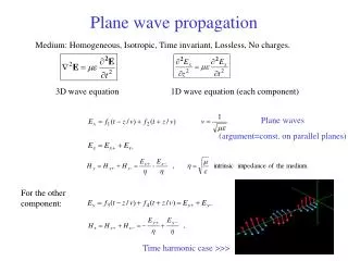
Plane wave propagation in a dielectric medium 1. Plane wave in a lossless homogeneous dielectric. The wave number for the wave propagating in a vacuum is a function of permittivity and permeability of free space: (7.37.1) Naturally, for a dielectric medium that may have different constants, the wave number will be (7.37.2)
Plane wave propagation in a dielectric medium If a plane wave generated by a signal generator propagates through two different dielectrics… Say, with the same magnetic constants but different permittivities, the wave numbers will be for these two media: (7.38.1) Both signals travel the same distance z but will have different phase velocities: (7.38.2)
Plane wave propagation in a dielectric medium This difference in velocities delays the arrival of one signal with respect to the other and causes a phase difference that can be detected: (7.39.1) If the total phase change in the signal passing through one of the paths is known: (7.39.2) The relative phase difference is (7.39.3) Therefore, if the properties of one of the regions are known and the phase difference is measured, we can identify the other material.
Plane wave propagation in a dielectric medium The ratio of the phase velocity in a vacuum to the phase velocity in a dielectric is called the index of refraction for the material: (7.40.1) Optical materials are usually characterized by their index of refraction.
Plane wave propagation in a dielectric medium Example 7.7: Find the phase difference if one region is filled with a gas with r = 1.0005 and the other region is a vacuum. The frequency of oscillation is 10 GHz and the length is z = 1m. The phase difference is This difference is small but can be detected. Also, if the travel distance is increased, the resolution (i.e. detectable phase difference) will be higher.
Plane wave propagation in a dielectric medium 2. Plane wave in a lossy homogeneous dielectric. A dielectric material can be lossy, i.e. exhibit a nonzero conductivity . In this situation, a conduction current must be added to the displacement current when considering the Ampere’s law. (7.42.1) (7.42.2) Assuming, as before, no free charges (v= 0) and following the same procedure: (7.42.3)
Plane wave propagation in a dielectric medium Assuming, as previously, that the electric field is linearly polarized in the y direction and the wave propagates in the z direction, we arrive to: (7.43.1) or (7.43.2) Where the propagation constant: (7.43.3)
Plane wave propagation in a dielectric medium The propagation constant is complex: (7.44.1) In a vacuum, = 0 and = k. In a general case, the real and imaginary parts are nonlinear functions of the frequency: (7.44.2) (7.44.3)
Plane wave propagation in a dielectric medium As a result, the phase velocity may depend on the wave’s frequency. This phenomena is called dispersion and the medium in which wave is propagating, is called a dispersive medium (every lossy medium). (7.45.1) Another quantity we recall here is the group velocity: (7.45.2)
Plane wave propagation in a dielectric medium The component of the electric field propagating in the +z direction is: (7.46.1) Wave propagates with a phase constant but the amplitude decreases with an attenuation constant . Units of are radians/m. Units of are nepers/m [Np/m]. If = 1 Np/m, the amplitude of the wave will decrease e times at a distance 1 m. 1 Np/m 8.686 dB/m. The characteristic impedance is: (7.46.2)
Plane wave propagation in a dielectric medium Example 7.8: A 10 V/m wave at the frequency 300 MHz propagates in the +z direction in an infinite medium. The electric field is polarized in the x direction. The parameters of medium are r = 9, r = 1, and = 10 S/m. Write the complete time domain expression for the electric field. We can find the attenuation constant as The phase constant is:
Plane wave propagation in a dielectric medium The complex propagation constant is 108 + j110 and the electric field is Example 7.9: Plot the phase velocity and the group velocity for the medium with r = 9, r = 1, and = 10 S/m The velocities can be described by (7.45.1) and (7.45.2). Both velocities increase with the frequency. The limit is the same:
Plane wave propagation in a dielectric medium Two approximations are frequently used: A) A dielectric with small losses ( << ) with a high-frequency approximation: (7.49.1) The approximate values for attenuation and propagation constants are: (7.49.2) (7.49.3)
Plane wave propagation in a dielectric medium (7.50.1) In this situation, the phase and the group velocities are the same. Also, some attenuation is introduced. “A pizza in a microwave oven”: water in the pizza acts as a conductor turning pizza into a complex impedance. The wave passing through it decays, therefore, the energy is absorbed and must be converted into heat. B) A dielectric with large losses ( >> ) with a low-frequency approximation: The conduction current is much greater than the displacement current, therefore: (7.50.2)