Estimation of Prevalence and Odds Ratios in Surveys
170 likes | 195 Vues
Learn how to estimate prevalence and odds ratios in surveys, covering confidence levels, error types, sample size calculations, and comparison methodologies.

Estimation of Prevalence and Odds Ratios in Surveys
E N D
Presentation Transcript
Surveys Sample Size By R. Heberto Ghezzo Ph.D. Meakins-Christie laboratories McGill University - Montreal - Canada
Objective of the Study Estimation Prevalence Odds- Ratio [Relative Risk if Cohort] Comparison Prevalence Odds-ratios [Relative Risk if Cohort]
Estimation • Confidence level - 90 %; 95 %; 99 % • Acceptable width of interval - 1 %, 5 %, 10 %, 20 %
Comparison • Error type 1 - alpha - 0.05 ; 0.01 • Smallest difference worth detecting - delta • Error type 2 - beta - 0.10 ; 0.05 ; 0.01
Error type 1 - alpha Error in claiming a difference when there is none. Alpha percent of normal people are thus classified into “abnormal”
Error type 2 - beta Error of not finding a difference when the difference is greater than the threshold or value of delta. Depends on the definition of the threshold i.e. the difference worth detecting, delta .
Which size? In surveys the errors are generally the same i.e. alpha = beta The level depends on the importance of the issue. Critical studies use beta=0.01
Estimation of a Prevalence n = z21-a/2 p(1 - p) / d2 n = z21-a/2 (1 - p) / e2 p a = error type 1 - alpha d = absolute width of conf.interval e = relative width of conf.interval
Estimation of an Odds-Ratio n = z21-a/2 {1/p1(1-p1) + 1/p2(1-p2)} / ln2(1-e) a = error type 1 - alpha e = relative width of conf.interval p1 = proportion exposed in cases p2 = proportion exposed in controls. OR = p1(1-p2)/(1-p1)p2
Estimation of a Relative Risk n = z21-a/2 {(1-p1)/p1 + (1-p2)/p2} / ln2(1-e) a = error type 1 - alpha e = relative width of conf.interval p1 = proportion exposed in cases p2 = proportion exposed in controls. RR = p1/p2
Comparing 2 prevalence n = {z1-a/22p(1-p) + z1-b p1(1-p1)+p2(1-p2)}2/(p1-p2)2 If p < 0.05 N = (z1-a/2 + z1-b)2 / [0.00061(arcsin p2 - arcsin p1)2] b = beta = 1-Power p = (p1 + p2)/2
Testing Odds Ratio > 1.0 n = {z1-a/22p2(1-p2) + z1-b p1(1-p1)+p2(1-p2)}2/(p1-p2)2 p1 = prevalence of exposure in cases p2 = prevalence of exposure in controls b = beta = 1-Power
Total Sample Size If design is stratified and tests/estimations will be done at each strata. The sample size applies to each strata. Otherwise all within strata comparisons or estimations will have larger errors or confidence intervals.
True Size I These formulae are theoretical. No real variable is truly normal. The estimator of variability has its own variability. There is no guarantee that the precision postulated will be achieved.
True Size II The estimator of variability comes from a different study. If the variability of the proposed study is larger the precision will deteriorate. Always use a beta error smaller than really needed and adjust the sample size upwards to a round number.
Non Response The sample size refers to the number of complete responses needed. Non response must be estimated and taken into account to arrive to the final size
Imputation To impute is to fake a value that does not exist Only to complete observations for a multivariate technique
