Download

1 / 39
600 likes | 1.54k Vues
CLASS NOTES HANDOUT VERSION. 4.1c Further Mechanics SHM & Oscillations. Breithaupt pages 34 to 49. January 4 th 2012. AQA A2 Specification. Oscillations (definitions). An oscillation is a repeated motion about a fixed point.

E N D
CLASS NOTES HANDOUT VERSION 4.1c Further MechanicsSHM & Oscillations Breithaupt pages 34 to 49 January 4th 2012
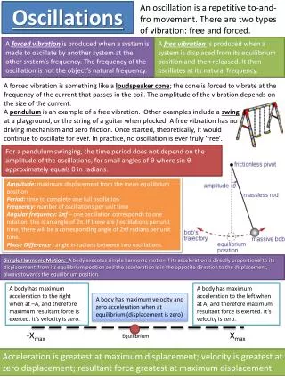
Oscillations (definitions) An oscillation is a repeated motion about a fixed point. The fixed point, known as the equilibrium position, is where the oscillating object returns to once the oscillation stops. The time period, Tof an oscillation is the time taken for an object to perform one complete oscillation. equilibrium position
equilibrium position The amplitude, A of an oscillation is equal to the maximum value of the displacement, x Frequency, f in hertz is equal to the number of complete oscillations per second. also: f = 1 / T Angular frequency, ω in radians per second is given by: ω= 2π f or ω= 2π / T
Many oscillating systems undergo a pattern of oscillation that is, or approximately the same as, that known as Simple Harmonic Motion (SHM). Examples (including some that are approximate): A mass hanging from the end of a spring Molecular oscillations A pendulum or swing A ruler oscillating on the end of a bench The oscillation of a guitar or violin string Tides Breathing Simple Harmonic Motion
The pattern of SHM is the same as the side view of an object moving at a constant speed around a circular path The pattern of SHM motion The amplitude of the oscillation is equal to the radius of the circle. + A The object moves quickest as it passes through the central equilibrium position. - A The time period of the oscillation is equal to the time taken for the object to complete the circular path.
When an object is performing SHM: 1. Its acceleration is proportional to its displacement from the equilibrium position. 2. Its acceleration is directed towards the equilibrium position. Mathematically the above can be written: a = - k x where k is a constant and the minus sign indicates that the acceleration, a and displacement, x are in opposite directions Conditions required for SHM
The constant k is equal to(2πf )2 or ω2 or (2π/T)2 Therefore: a = - (2πf )2 x(given on data sheet) or a = - ω2 x or a = - (2π/T)2 x a + ω2 x x - A + A - ω2 x Acceleration variation of SHM gradient = - ω2 or - (2πf )2
A body oscillating with SHM has a period of 1.5s and amplitude of 5cm. Calculate its frequency and maximum acceleration. Question
The displacement, x of the oscillating object varies with time, t according to the equations: x = A cos (2π f t) given on data sheet or x = A cos (ω t) or x = A cos ((2π / T) t) Note: At time, t = 0, x = +A Displacement equations of SHM
A body oscillating with SHM has a frequency of 50Hz and amplitude of 4.0mm. Calculate its displacement and acceleration 2.0ms after it reaches its maximum displacement. Question
The velocity, v of an object oscillating with SHM varies with displacement, x according to the equations: v = ± 2πf √(A2 − x 2) given on data sheet or v = ± ω√(A2 − x 2) or v = ± (2π / T) √(A2 − x 2) Velocity equations of SHM
Question A body oscillating with SHM has a period of 4.0ms and amplitude of 30μm. Calculate (a) its maximum speed and (b) its speed when its displacement is 15μm.
Variation of x, v and a with time The acceleration, ax depends on the resultant force, Fspring on the mass. Note that the acceleration ax is always in the opposite direction to the displacement, X.
SHM time graphs - A + A T/4 T/2 3T/4 T 5T/4 3T/2 x x v a time v a x = A cos (2π f t) v = - 2π f A sin (2π f t) vmax = ± 2π f A a = - (2π f )2 A cos (2π f t) amax = ± (2π f )2 A Note: The velocity curve is the gradient of the displacement curve and the acceleration curve is the gradient of the velocity curve.
SHM graph question T/4 T/2 3T/4 T 5T/4 3T/2 The graph below shows how the acceleration, a of an object undergoing SHM varies with time. Using the same time axis show how the displacement, x and velocity, v vary in time. a time
If a mass, m is hung from a spring of spring constant, k and set into oscillation the time period, T of the oscillations is given by: T = 2π√(m / k) AS Reminder:Spring Constant, k: This is the force in newtons required to cause a change of length of one metre. k = F / ΔL unit of k = Nm-1 The spring-mass system Mass on spring - Fendt
A spring extends by 6.0 cm when a mass of 4.0 kg is hung from it near the Earth’s surface (g = 9.8ms-2). If the mass is set into vertical oscillation state or calculate the period (a) near the Earth’s surface and (b) on the surface of the Moon where g = 1.7 ms-2. Question
A simple pendulum consists of: a point mass undergoing small oscillations (less than 10°) suspended from a fixed support by a massless,inextendable thread of length, L within a gravitational field of strength, g The time period, T is given by: T = 2π√(L / g) The simple pendulum • Simple Pendulum - Fendt
Calculate: (a) the period of a pendulum of length 20cm on the Earth’s surface (g = 9.81ms-2) and (b) the pendulum length required to give a period of 1.00s on the surface of the Moon where g = 1.67ms-2. Question
A freely oscillating object oscillates with a constant amplitude. The total of the potential and kinetic energy of the object will remain constant. EP + ET = a constant This occurs when there are no frictional forces acting on the object such as air resistance. Free oscillation
Energy variation in free oscillation 1 5 2 4 3 equilibrium position
A simple pendulum consists of a mass of 50g attached to the end of a thread of length 60cm. Calculate: (a) the period of the pendulum (g = 9.81ms-2) and (b) the maximum height reached by the mass if the mass’s maximum speed is 1.2 ms-1. Question
The strain potential energy is given by: EP = ½ k x2 Therefore the maximum potential energy of an oscillating spring system = ½ k A2 = Total energy of the system, ET But: ET = EP + EK ½ k A2 = ½ k x2 + EK And so the kinetic energy is given by: EK = ½ k A2 - ½ k v2 EK = ½ k (A2 - x2) Energy variation with an oscillating spring
The potential energy curve is parabolic, given by: EP = ½ k x2 The kinetic energy curve is an inverted parabola, given by: EK = ½ k (A2 - x2) The total energy ‘curve’ is a horizontal line such that: ET = EP+EK energy - A 0 + A displacement, x Energy versus displacement graphs ET EK EP
Displacement varies with time according to: x = A cos (2π f t) Therefore the potential energy curve is cosine squared, given by: EP = ½ k A2 cos2 (2π f t) ½ k A2= total energy, ET. and so: EP = ET cos2 (2π f t) Kinetic energy is given by: EK=ET-EP EK=ET-ET cos2 (2π f t) EK=ET(1 -cos2 (2π f t)) EK = ETsin2 (2π f t) EK = ½ k A2sin2 (2π f t) energy ET ½ kA2 EP EK 0 T/4 T/2 3T/4 T time, t Energy versus time graphs
Damping occurs when frictional forces cause the amplitude of an oscillation to decrease. The amplitude falls to zero with the oscillating object finishing in its equilibrium position. The total of the potential and kinetic energy also decreases. The energy of the object is said to be dissipated as it is converted to thermal energy in the object and its surroundings. Damping
1. Light Damping In this case the amplitude gradually decreases with time. The period of each oscillation will remain the same. The amplitude, A at time, t will be given by: A = A0 exp (- C t) where A0 = the initial amplitude and C = a constant depending on the system (eg air resistance) Types of damping
2. Critical Damping In this case the system returns to equilibrium, without overshooting, in the shortest possible time after it has been displaced from equilibrium. 3. Heavy Damping In this case the system returns to equilibrium more slowly than the critical damping case. displacement A0 time critical damping heavy damping light damping
Forced oscillations All undamped systems of bodies have a frequency with which they oscillate if they are displaced from their equilibrium position. This frequency is called the natural frequency, f0. Forced oscillation occurs when a system is made to oscillate by a periodic force. The system will oscillate with the applied frequency, fA of the periodic force. The amplitude of the driven system will depend on: 1. The damping of the system. 2. The difference between the applied and natural frequencies.
Resonance The maximum amplitude occurs when the applied frequency, fA is equal to the natural frequency, f0 of the driven system. This is called resonanceand the natural frequency is sometimes called the resonant frequency of the system.
Resonance curves amplitude of driven system, A very light damping light damping more damping driving force amplitude f0 applied force frequency, fA
Notes on the resonance curves If damping is increased then the amplitude of the driven system is decreased at all driving frequencies. If damping is decreased then the sharpness of the peak amplitude part of the curve increases. The amplitude of the driven system tends to be: - Equal to that of the driving system at very low frequencies. - Zero at very high frequencies. - Infinity (or the maximum possible) whenfA is equal to f0 as damping is reduced to zero.
Phase difference The driven system’s oscillations are always behind those of the driving system. The phase difference lag of the driven system depends on: 1. The damping of the system. 2. The difference between the applied and natural frequencies. At the resonant frequency the phase difference is π/2 (90°)
Phase difference curves - 90° more damping less damping - 180° f0 applied force frequency, fA phase difference of driven system compared with driving system
Examples of resonance • Pushing a swing • Musical instruments (eg stationary waves on strings) • Tuned circuits in radios and TVs • Orbital resonances of moons (eg Io and Europa around Jupiter) • Wind driving overhead wires or bridges (Tacoma Narrows)
The Tacoma Narrows Bridge Collapse YouTube Videos: http://www.youtube.com/watch?v=3mclp9QmCGs – 4 minutes – with commentary http://www.youtube.com/watch?v=IqK2r5bPFTM&feature=related – 3 minutes – newsreel footage http://www.youtube.com/watch?v=j-zczJXSxnw&feature=related – 6 minutes - music background only An example of resonance caused by wind flow. Washington State USA, November 7th 1940.