Download

1 / 26
270 likes | 639 Vues
Nonlinear Oscillations; Chaos Chapter 4. All oscillators treated so far were Linear Oscillators: Obey Hooke’s “Law”. The restoring force is linear: F(x)= -kx Potential energy U(x) = (½)kx 2 Real world: Most oscillators are, in fact, nonlinear!

E N D
Nonlinear Oscillations; ChaosChapter 4 • All oscillators treated so far were Linear Oscillators: Obey Hooke’s “Law”. The restoring force is linear:F(x)= -kx Potential energyU(x) = (½)kx2 • Real world: Most oscillators are, in fact, nonlinear! • Techniques for solving linear problems might or might not be useful for nonlinear ones! • Often, rather than having a general technique for nonlinear problem solution, the technique to use may be problem dependent. • Often (almost always) numerical techniques are needed to solve the differential equations.
Most oscillators are nonlinear! • Many techniques exist for solving (or at least approximately solving) nonlinear diff. eqtns. • Often, nonlinear systems reveal a rich & beautiful physics that is simply not there in linear systems. (e.g. Chaos). • The related areas of nonlinear mechanics and Chaos are very modern and are (in some places) hot topics of current research. • I am not an expert!
Consider a general one dimensional, driven, damped oscillator for which the Newton’s 2nd Law equation of motion is: [a = (d2x/dt2); v = (dx/dt)] ma + f(v)+ g(x) = h(t) (1) • f(v), g(x), h(t) areproblem dependent! • If f(v) contains powers of v higher than linear & / or g(x) contains powers of x higher than linear, (1) is a non-linear differential equation! • Complete, general solutions are not always available! • Sometimes a special treatment adapted for the problem is needed. • We can often learn a lot by considering deviations from linearity. • Sometimes examining (v –x) phase diagrams is useful.
Brief history & terminology(see interesting historical footnotes): • Early 1800’s: Laplace’s idea: Newton’s 2nd Law: If at t = 0 the positions & velocities of all particles in universe were known, & if the force laws governing particle interactions were known, then we can know the exact future of the universe by integrating Newton’s 2nd Law equations. • This is the deterministic view of nature. • Recently, especially in past 30-35 years, researchers in many (very different) areas of science have realized that knowing the laws of nature is not enough. Much of nature is chaotic!
Chaos • Terminology: • Deterministic Chaos:Motion of a system whose time evolution depends sensitively on the initial conditions. • Deterministic:For given initial conditions, Newton’s 2nd Law equations give the exact future of the system. • Chaos: Only slight changes in initial conditions can result in drastic changes in the system motion. • Random: There is no correlation between the system’s present state & its immediate past state. CHAOS & RANDOMNESS ARE DIFFERENT!
Chaos:Measurements on the system at a given time might not allow the future to be predicted with certainty, even if the force laws are known exactly!(For example, experimental uncertainties in the initial conditions could lead to very different behavior than predicted by N’s 2nd Law.) • Deterministic Chaos:Alwaysassociated with a system nonlinearity. • Nonlinearity: Necessary for chaos, but not sufficient! All chaotic systems are nonlinear but not all nonlinear systems are chaotic! • Chaos occurs when the system state depends in a very sensitive way on its previous state. Even a tiny change in the conditions can completely (qualitatively & quantitatively) change the system motion.
Chaotic Systems: • The equations of motion can only be solved numerically. • Only with the availability of modern computers has it become possible to study these phenomena. • There are (unfortunately) no simple, general rules for when a system will be chaotic or not. • SOME chaotic phenomena in the real world: Irregular heartbeats; planetary motion in the solar system(!); some electrical circuits; weather patterns …...
Chaotic Systems: • Henri Poincaré: In the late 1800’s. Was the first to recognize chaos (in celestial mechanics). • Real breakthroughs in understanding didn’t come until the 1970’s (with computers). • Chaos study is widespread. Here, we will only give a brief, elementary introduction. • Many textbooks and popular texts exist! See the references & bibliography! • This is a popular & popularized topic even in the mainstream, popular press.
Nonlinear OscillationsSection 4.2 • Consider a parabolic, 1d potential energy: U(x) = (½)kx2 Force: F = - (dU/dx) = - kx Obviously, this is the case of the simple (linear) harmonic oscillator, already discussed in great detail! • Consider a more general (complicated) 1d potential energy: U(x) The force is still: F = - (dU/dx)
Consider a general 1d potential U(x),F = - (dU/dx). Let U(x) have local minimum, Uminat x = 0, as shown: Assume a mass m has energy E, & is confined to a region not too far from x = 0 (between 2 turning points). E x = 0
m can’t get too far away from x = 0, so make a Taylor’s series expansion of U(x) about x = 0: U(x) Umin + x(dU/dx)0 + (1/2!)x2(d2U/dx2)0 + (1/3!)x3(d3U/dx3)0 + (1/4!)x4(d4U/dx4)0 + ….. • The zero of energy is arbitrary Often take Umin= 0 • The force at the equilibrium (x=0) position is 0 by the definition of equilibrium: F0 - (dU/dx)0 = 0 U(x) x2(d2U/dx2)0 + x3(d3U/dx3)0 + (1/24)x4(d4U/dx4)0 + • Define:k (d2U/dx2)0, -2λ (d3U/dx3)0, -6ε (d4U/dx4)0 U(x) kx2 - λx3 - εx4 + … F(x) -(dU/dx) = - kx + λx2 + εx3 + …
If (as we assume, as in the figure) the total energy E = T+U is very close to Umin, The displacement x from equilibrium is small & U(x) kx2& F(x) - kx • This is the linear (harmonic) oscillator problem we just did! • However, if the total energy E = T+U is large compared to Umin, The displacement x is not small & we must go to higher terms in the expansion F(x) will have nonlinear terms Newton’s 2nd Law will be a nonlinear differential equation!
For many common physical situations, U(x) is symmetric about equilibrium (x = 0) The coefficients of the odd powers of x in the Taylor’s series for U vanish (odd order derivatives of U = 0 at x = 0) (λ = 0). In this case, the magnitude of the force is the same at x & -x, but the direction is opposite. • In this situation: U(x) kx2 - εx4 + … F(x) - (dU/dx) = - kx + εx3 + …
Some terminology: • Consider such a symmetric potential: U(x) kx2 - εx4 F(x) - (dU/dx) = - kx + εx3 • Depending on the sign of ε - (d4U/dx4)0 , it’s possible that |F(x)| > |Flinear| or |F(x)| < |Flinear|, where Flinear = - kx (Hooke’s “Law” force). If ε > 0 , |F(x)| < |Flinear| & the system is “SOFT” If ε < 0 , |F(x)| > |Flinear| & system is “HARD”
U(x) kx2 - εx4 & F(x) -kx + εx3 for SOFT (ε > 0) & HARD (ε < 0) systems
This example discusses an intrinsicallynonlinear system, even though the forces involved are linear, Hooke’s “Law” forces! • A particle, mass m, is suspended between 2 springs (constants k, relaxed lengths , stretched lengths s). Find the steady state solution x(t) for a driving force F(t) = F0cos(ωt)(neglect gravity!) Example 4.1
Each spring exerts a linear, Hooke’s “Law” force on m equal to (see diagram) Fs = -k(s - ). Vector forces! Total vertical force vanishes (y components cancel). The total horizontal force is: F = -2k(s - ) sinθ • From geometry & trig, s = [2 +x2]½ sinθ = (x/s) = (x)/[2 +x2]½ • Putting this all together, (messy!) the horizontal force is (algebra):F(x) = -2kx (1- [1 +(x/)2]-½) • Assume (x/) is small: Expand F(x) in a Taylor’s series, keep only the first non-zero term & find: F(x) -(k/2)x3
This is an intrinsicallynonlinear system because even for very small amplitude (x) motion, the force is nonlinear! F(x) -(k/2)x3 • Could solve the Newton’s 2nd Law eqtn numerically (or otherwise?). But cannot easily contrast the solution with the linear oscillator since there is no linear force term! • In many problems, we are interested in results where the deviation from linearity is small. Can’t look at this either! • However, consider slightly different problem. The same picture, but this time, when vertical, the springs are not relaxed. Each needs to stretch a distance d from their relaxed lengths (0) to attach to mass m.
That is, = 0 + d • In problem 4.1 (to be assigned) it is shown, in this case: F(x) = -2kx{1- [(-d)/] [1 +(x/)2]-½} • Assume (x/) is small: Expand F(x) in a Taylor’s series & keep the first two non-zero terms: F(x) -2[(kd)/()]x -[k(-d)/(3)]x3 Both a linear & a non-linear term!
F(x) -2[(kd)/()]x -[k(-d)/(3)]x3 In the general notation of earlier: F(x) - kx + εx3 Can identify the parameters of the general discussion with the parameters for this case: k 2[(kd)/()] ε -[k(-d)/(3)] < 0 From the general discussion, the system is hard • Consider the Newton’s 2nd Law equation (with a sinusoidal driving force F0cos(ωt)): m(d2x/dt2) = F(x) + F0cos(ωt) or: m(d2x/dt2) = -2[(kd)/()]x - [k(-d)/(3)]x3 + F0cos(ωt)
New notation: G F0/m;ε -[k(-d)/(3)] a (2kd)/(m) • The differential equation is: (d2x/dt2) = - ax + εx3 + G cos(ωt) A very difficult equation to solve! (Can’t be done in closed form.) • We can, however, find many important characteristics of the solution x(t), especially where the deviation from linearity is small: (|εx3|<< |ax|) by using the Method of Successive Approximations(Perturbation Theory)
(d2x/dt2) = - ax + εx3 + G cos(ωt) (1) Method of Successive Approximations (outline): • Assume the nonlinear term is “small” (|εx3| << |ax|) Expect a solution like: x(t) xd(t) + small corrections where xd(t) = solution to the driven linear oscillator (from Ch. 3) 1st approximation ( x1(t)): Take the linear oscillator form, neglecting the nonlinear term completely. Assume: x1(t) = A cos(ωt) (Steady state term!) • 2nd approximation ( x2(t)): Obtained by using x1(t) on the right side of (1), letting x on left side be x2(t) & integrating twice:(d2x2/dt2) = - ax1 + εx13 + G cos(ωt)
(d2x2/dt2)= - ax1 + εx13 + G cos(ωt); x1(t) = A cos(ωt) (d2x2/dt2) = (G - aA) cos(ωt) + εA3 cos3(ωt) Trig identity: cos3(ωt) = cos(ωt) + cos(3ωt) So: (d2x2/dt2)= (G - aA+ εA3)cos(ωt) + εA3 cos(3ωt) • Integrate twice (there are 2 constants of integration, which depend on the initial conditions; take these as 0 here for simplicity): x2(t) = ω-2(G - aA+ εA3)cos(ωt) - ω-2[(εA3)/(36)]cos(3ωt)
x2(t) = ω-2(G - aA+ εA3)cos(ωt) - ω-2[(εA3)/(36)]cos(3ωt) (2) • Now, could continue with a 3rd approximation( x3(t)): Obtained by using x2(t) on the right side of (1) & letting x on left side be x3(t) & integrating twice: (d2x3/dt2 ) = - ax2 + εx23 + G cos(ωt) (clearly a mess!) • To get the correct, converged, detailed solution, we need the computer. • Even the result x2(t) is complicated! • A detailed discussion of this solution, its methods & numerics is beyond the scope of the course!
The authors qualitatively discuss the numerical iteration solution, & mention some interesting results obtained, which are all totally unexpected & unusualif one“thinks linearly” & is used to only linear equation results & solutions. However, they are not unusual for nonlinear systems! • The amplitude depends on driving frequency ω, but no resonance at natural frequency of system! • For some values of ω, 3 different amplitudes may occur, with discontinuous “jumps” (as function of ω) between them. • The amplitude for a given ωmay depend on whether ω is increasing or decreasing (the system displays hysteresis) • More on these kind of effects later!