Optimizing Ice Cream and Yogurt Production for Maximum Profit
Gillian’s Restaurant faces a challenge in managing its ice cream and yogurt production under capacity limits and budget constraints. The freezer can hold a maximum of 115 gallons, and the restaurant allocates $90 weekly for purchasing these products. The demand for ice cream is at least twice that of yogurt, and the profit margins are $4.15 and $3.60 per gallon, respectively. This analysis explores the optimal solution for production levels, examines cost sensitivity, and evaluates the impact of production adjustments on profitability.

Optimizing Ice Cream and Yogurt Production for Maximum Profit
E N D
Presentation Transcript
Gillian’s RestaurantCHP.2 Problem 34 & 35 • Two products, ice cream and yogurt • The freezer capacity is at most 115 gallons. • A gallon of ice cream costs $0.93 and a gallon of frozen yogurt costs $0.75. • Restaurant budgets $90 each week for these products. • The demand for ice cream is at least twice of the demand for frozen yogurt. • Profit per gallon of ice cream and yogurt are $4.15 and $3.60 , respectively.
Sensitivity Analysis REDUCED COST A decision variable with a positive value in the optimum solution will generally have zero reduced cost. Likewise, a decision variable with value zero in the optimum solution will have a non-zero reduced cost. The value of reduced cost gives the amount by which the objective function coefficient of this variable must change for this variable to have a non-zero value in the optimal solution
SENSITIVITY ANALYSIS SHADOW PRICE (DUAL VALUE) • It is the marginal value of increasing the right-hand side of any constraint. • binding constraints have zero slack or zero surplus and vice versa. • Shadow price for not binding constraints is zero. • Lower and upper bounds given for each constraint provide the range over which the shadow price for that constraint is valid.
SENSITIVITY ANALYSIS Dual ValueRHSmax Z (Profit)min Z (Cost) Positive increase increase decrease Positive decrease decrease increase Negative increase decrease increase Negative decrease increase decrease Note: As long as increases/decreases in RHSs are within the given lower and upper bounds
EXAMPLE 1 Tucker Inc. needs to produce 1000 Tucker automobiles. The company has four production plants. Due to differing workforces, technological advances, and so on, the plants differ in the cost of producing each car. They also use a different amount of labor and raw material at each. This is summarized in the following table: Plant Cost ('000) Labor Material 1 15 2 3 2 10 3 4 3 9 4 5 4 7 5 6 The labor contract signed requires at least 400 cars to be produced at plant 3;there are 3300 hours of labor and 4000 units of material that can be allocated to the four plants.
Questions for Example 1 1. What is the optimum solution? What is the current cost of production? 2. How much will it cost to produce one more vehicle? How much will we save by producing one less? 3. How would our solution change if it costs only $8,000 to produce at plant 2? 4. For what ranges of costs is our optimal solution (except for the objective value) valid for plant 2? 5. How much are we willing to pay for one more labor hour?
Questions for Example 1 6. What would be the effect of reducing the 400 car limit down to 200 cars? To 0 cars? What would be the effect of increasing it by 100 cars? by 200 cars? 7. How much is our raw material worth (to get one more unit)? How many units are we willing to buy at that price? What will happen if we want more?