Modeling Quantities Changing at Constant Rates
Learn to model changing quantities with linear functions and equations. Study piecewise-defined functions and the greatest integer function. Explore direct variation and solve problems using Hooke's Law.

Modeling Quantities Changing at Constant Rates
E N D
Presentation Transcript
Chapter 2 Linear Functions and Equations
More Modeling with Functions 2.4 Model data with a linear function Evaluate and graph piecewise-defined functions Evaluate and graph the greatest integer function Use direct variation to solve problems
Modeling with Linear Functions To model a quantity that is changing at a constant rate with f(x) = ax + b, the following formula may be used. f(x) = (constant rate of change)x + initial amount The constant rate of change corresponds to the slope of the graph of f, and the initial amount corresponds to the y-intercept.
A 100-gallon water tank, initially full of water, is being drained at a rate of 5 gallons per minute. Example: Finding a symbolic representation (a) Write a formula for a linear function f that models the number of gallons of water in the tank after x minutes. (b) How much water is in the tank after 4 minutes? (c) Graph f. Identify the x- and y-intercepts and interpret each. (d) Discuss the domain of f.
(a) Water in tank decreasing at 5 gal/min, so constant rate of change is –5. The initial amount of water is 100 gal. Example: Finding a symbolic representation Solution (b) After 4 min the tank contains:
(c) Slope: –5y-intercept: 100 - the number of gallons of water initially in the tankx-intercept: 20 - time in min to empty the tank Example: Finding a symbolic representation
(d) From the graph: the domain of f must be restricted to 0 ≤ x ≤ 20. It makes sense: can’t have negative time, f(21) = –5(21) + 100 = –5tank can’t hold –5 gallons of water Example: Finding a symbolic representation
Piecewise-Defined Functions A function f that models data and is defined on pieces of its domain is called a piece-wise function. If each piece is linear, the functions is a piece-wise linear function.
Fujita Scale - Intensity of Tornadoes An F1 tornado has winds speeds between 40 and 72 miles per hour. Here is the piece-wise function for the F-scale.
Use f(x) to complete the following: Example: Evaluating and graphing a piecewise-defined function (a) What is the domain of f ? (b) Evaluate f(–3), f(2), f(4), and f(5). (c) Sketch a graph of f. (d) Is f a continuous function on its domain?
Solution Example: Evaluating and graphing a piecewise-defined function (a) f is defined for –4 ≤ x < 2 or 2 ≤ x ≤ 4 domain is D = {x |–4 ≤ x ≤ 4}, or [–4, 4] (b) f(–3) = –3 – 1 = –4f(2) = –2 • 2 = –4f(4) = –2 • 4 = –8f(5) is undefined (5 is not in the domain)
Example: Evaluating and graphing a piecewise-defined function (c) Sketch a graph of f. From –4 up to 2, graphy = x – 1, open circle at 2 From 2 to 4, graphy = –2x (d) f is not continuousbecause there is a break at x = 2
Greatest Integer Function The greatest integer functionis defined as follows. is the greatest integer less than or equal to x.
Direct Variation Let x and y denote two quantities. Then y is directly proportional to x, or y varies directly with x, if there exists a nonzero number k such that y = kx k is called the constant of proportionality or the constant of variation.
Hooke’s Law Hooke’s law states that the distance that an elastic spring stretchesbeyond its natural length is directly proportionalto the amount of weight hung on thespring, as illustrated in the Figure.
Hooke’s Law This law is valid whether the spring is stretched or compressed. The constant of proportionality is called the spring constant. Thus if a weight or force F is applied and the spring stretches a distance x beyond its natural length, then the equation F = kx models this situation, where k is the spring constant.
A 12-pound weight is hung on a spring, and it stretches 2 inches. Example: Working with Hooke’s law (a) Find the spring constant. (b) Determine how far the spring will stretch when a 19-pound weight is hung on it. Solution Let F = kx: F = 12 pounds, x = 2 inches F = k(2) so k = 6 The spring constant equals 6
Example: Working with Hooke’s law (b) F = 19
Solving a Variation Problem When solving a variation problem, the following steps can be used. STEP 1: Write the general equation for the type of variation problem that you are solving. STEP 2: Substitute given values in this equation so the constant of variation k is the only unknown value in the equation. Solve for k.
Solving a Variation Problem STEP 3: Substitute the value of k in the general equation in Step 1. STEP 4: Use this equation to find the requested quantity.
Let T vary directly with x, and suppose that T = 33 when x = 5. Find T when x = 31. Example: Solving a direct variation problem Solution STEP 1: Direct variation is T = kx STEP 2: Substitute 33 for T, 5 for x , solve for k
Example: Solving a direct variation problem STEP 3: STEP 4: When x = 31, we have: