Download
1 / 19
190 likes | 219 Vues
Explore the β effect on geostrophic flow rotation with depth using the thermal wind equation under Boussinesq approximation. Learn about wind-driven circulation and wind stress calculation for the ocean surface. Understand the Ekman layer near the sea surface and its three-way force balance.

E N D
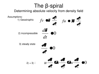
The β-spiralDetermining absolute velocity from density field Assumptions: 1) Geostrophic 2) incompressible 3) steady state 2) + 3)
Use the thermal wind equation with Boussinesq approximation Take into Write u and v to polar format as In the northern hemisphere, if w > 0, the current rotates to the right as we go upward (or to the left as we go downward)
Take geostrophic equation If v≠0, w changes with z and can not be zero everywhere. Thus the β effect makes the rotation of the geostrophic flow with depth likely, hence the term “β spiral” use
Consider an isopycnal surface at If we go along this surface in the x-direction Similarly Take into
Rewrite the thermal wind relation Suppose we have derived u’ and v’ based on some reference level If the observations should be error free, two levels would be sufficient Considering the observation errors, particularly noise from time-dependent motions, this equation will not be exactly satisfied. Computationally, a least-square technique is used.
Wind Driven Circulation I:Planetary boundary Layer near the sea surface
Surface wind stress • Approaching sea surface, the geostrophic balance is broken, even for large scales. • The major reason is the influences of the winds blowing over the sea surface, which causes the transfer of momentum (and energy) into the ocean through turbulent processes. • The surface momentum flux into ocean is called the surface wind stress ( ), which is the tangential force (in the direction of the wind) exerting on the ocean per unit area (Unit: Newton per square meter) • The wind stress effect can be constructed as a boundary condition to the equation of motion as
Wind stress Calculation • Direct measurement of wind stress is difficult. • Wind stress is mostly derived from meteorological observations near the sea surface using the bulk formula with empirical parameters. • The bulk formula for wind stress has the form Where is air density (about 1.2 kg/m3 at mid-latitudes), V (m/s), the wind speed at 10 meters above the sea surface, Cd, the empirical determined drag coefficient
Drag Coefficient Cd • Cd is dimensionless, ranging from 0.001 to 0.0025 (A median value is about 0.0013). Its magnitude mainly depends on local wind stress and local stability. • Cd Dependence on stability (air-sea temperature difference). More important for light wind situation For mid-latitude, the stability effect is usually small but in tropical and subtropical regions, it should be included. • CdDependence on wind speed.
Cd dependence on wind speed in neutral condition Large uncertainty between estimates (especially in low wind speed). Lack data in high wind
Annual Mean surface wind stress Unit: N/m2, from Surface Marine Data (NODC)
December-January-February mean wind stress Unit: N/m2, from Surface Marine Data (NODC)
June-July-August mean wind stress Unit: N/m2, from Surface Marine Data (NODC)
The primitive equation (1) (2) (3) (4) Since the turbulent momentum transports are , , etc We can also write the momentum equations in more general forms At the sea surface (z=0), turbulent transport is wind stress. ,
Assumption for the Ekman layer near the surface • Az=const • Steady state • Small Rossby number • Large vertical Ekman Number • Homogeneous water (ρ=const) • f-plane (f=const) • no lateral boundaries (1-d problem) • infinitely deep water below the sea surface
Ekman layer • Near the surface, there is three-way force balance Coriolis force+vertical dissipation+pressure gradient force=0 Take and let ( , ageostrophic (Ekman) current, note that is not small in comparison to in this region) then
The Ekman problem Boundary conditions At z=0, As z→-∞, ,. , . Let (complex variable) At z=0, As z→-∞,
The solution Assuming f > 0, the general solution is Using the boundary conditions, we have Set , where and note that