Download

1 / 18
180 likes | 311 Vues
Determining orientation, thickness and velocity for a 2D, non-planar magnetopause. A. Blăgău(1,2), B. Klecker(1), G. Paschmann(1), M. Scholer(1), S. Haaland(1,3), O. Marghitu(2,1), and E. A. Lucek(4) (1) Max-Planck-Institut fuer extraterrestrische Physik, Garching, Germany

E N D
Determining orientation, thickness and velocity for a 2D, non-planar magnetopause A. Blăgău(1,2), B. Klecker(1), G. Paschmann(1), M. Scholer(1), S. Haaland(1,3), O. Marghitu(2,1), and E. A. Lucek(4) (1) Max-Planck-Institut fuer extraterrestrische Physik, Garching, Germany (2) Institute for Space Sciences, Bucharest, Romania (3) Department of Physics, University of Bergen, Norway (4) Imperial College, London, UK
Introduction • The aim: • To show a timing-based method, developed for inferring the crossing parameters for a 2D, non-planar magnetopause (MP) • Outline: • Short description of the existing planar methods • One case of a 2D, non-planar MP will be presented • The new method, conceived to deal with such cases, will be introduced • Comparison of the results given by the planar methods and the results obtained with the new technique
Existing planar methods (selection) Crossing parameters: velocity, thickness and orientation of the MP (curvature) The planar methods relevant for this talk: • Minimum variance analysis of the magnetic field (MVA) • Sonnerup, B. and Scheible, M, ISSI Report, 1998 • Timing analysis (TA) • Haaland, S. et al. AnGeo, 22, 4, 2004 • Minimum Faraday residue (MFR) technique • Khrabrov, A.V. and Sonnerup, B.U.Ö, GRL, 25, 2373, 1998 • deHoffmann-Teller (HT) analysis • Khrabrov, A. V. and Sonnerup, B., ISSI Report, 1998 We shall illustrate these methods on a case of in-bound MP crossing at the dawn magnetospheric flank
Magnetic variance analysis • Single satellite method • The algorithm finds the direction in space along which the magnetic field recorded during the transition is roughly constant (along which its variance has a minimum) and associates it with the MP normal • The MP velocity is not found. For this we have to use other technique (like deHoffmann –Teller analysis) The MP crossing is put in evidence by the change in the magnetic field orientation Due to the presence of superimposed small-scale fluctuation, we used the constrained (to <Bn> = 0) MVA algorithm The normals are very well defined (a pronounced minimum in the magnetic variance was found). λmax/ λint > 130
Timing technique • Multi-spacecraft method. • Uses the differences in MP crossing times and crossing positions by the 4 Cluster satellite • There are two approaches in this technique: one assuming that the MP velocity is constant (CVA) and one that it has a constant thickness (CTA). • The crossing times should characterize the MP transition as a whole. Therefore we fitted the max. var. component with a tanh profile and picked the central points. • For establishing the crossing duration we adopted a convention about the MP extent (a fraction of tanh(1) ~ 76% of the total jump; horizontal dashed lines). • We obtained in this way the central crossing times (Tcentral) and the crossing duration (deltaT). Equivalently, we have the times when the satellite detects the MP leading and trailing edges.
Timing technique • Multi-spacecraft method. • Uses the differences in MP crossing times and crossing positions by the 4 Cluster satellite • There are two approaches in this technique: one assuming that the MP velocity is constant (CVA) and one that it has a constant thickness (CTA). The satellites are crossing the MP in pairs (C2-C4 followed by C3-C1) We obtained reliable timing information due to the regular signature in the magnetic field data for each satellite
Minimum Faraday residue technique • Single spacecraft technique • The algorithm finds a direction in space and a velocity (assumed constant) along this direction for which the tangential component of the electric field is roughly constant • The electric field data for this event are not so good. Still, the MFR method could be used as comparison • The crossing durations (established in the TA) are indicated by the vertical solid lines. The vertical dotted lines indicate the Interval used in MFR analysis
deHoffmann – Teller analysis Results from the HT analysis • Single-spacecraft method • Search for the existence of a reference system in which the convection electric field is zero (search whether the data corresponding to the MP transition could be interpreted as produced by time-stationary structure, without an intrinsic electric field, moving over the spacecraft) • The velocity of the reference frame is searched. When the test is successful, the component of this velocity along the MP normal is associated with the MP velocity • For the electric field, we used the approximation E= -v X B in case of Cluster 1, 3 and 4. For Cluster 2 we used directly the electric field measurements. • The ‘goodness of the test’ is express in the correlation between the E in satellite SC and the convection E produced by a movement with VHT • In our case the MP possesses a fairly good deHoffmann-Teller frame.
Normals orientation • The orientation of the normals are shown in a polar plot • The center represents a reference direction in space (average of the individual MVA normals, shown in colors) • The circles designate directions of equal inclination, in degrees • The MVA normals are grouped in pairs because the satellites are crossing the MP in pairs • Note that the two groups of normals are well separated (approx. 12 degrees) • Due to the well-defined MVA normals for this particular transition, this can not be explained by the second order effects (noise, waves, experimental errors etc.) • We conclude that the MP is non-planar
Normals orientation • The orientation of the normals are shown in a polar plot • The center represents a reference direction in space (average of the individual MVA normals, shown in colors) • The circles designate directions of equal inclination, in degrees • The MVA normals lie roughly in one plane (dashed line) • This suggests that Cluster encountered a 2D, non-planar MP with the invariant direction perpendicular to that plane (magenta arrow) • From the MVA theory we knew that the results are influenced by the non-planarity, but for a 2D MP the normals will still be contained in the plane perpendicular to
Normals orientation • The orientation of the normals are shown in a polar plot • The center represents a reference direction in space (average of the individual MVA normals, shown in colors) • The circles designate directions of equal inclination, in degrees • The same plot with an increased direction range, to include the TA normals • Despite the accurate timing information, the CVA and CTA normals are well apart the MVA normals • Because now we rely on the timing and satellite positions (not directly on the actual data) a 2D MP will not produce, in general, normals in the plane perpendicular to Another indication that the planar assumption is not appropriate for this case
Normals orientation • The orientation of the normals are shown in a polar plot • The center represents a reference direction in space (average of the individual MVA normals, shown in colors) • The circles designate directions of equal inclination, in degrees • The MFR normals (coloured dots), although not as reliable as MVA normals, are close to the plane perpendicular to the invariant direction (below 5 degrees) • As in the case of MVA method, for an ideal 2D MP the normals will lie in the plane perpendicular to (although their orientation will be influenced by the non-planar effects)
The 2-D model • We modelled the MP as a 2D layer, having a constant thickness and oriented along the invariant direction • Two geometries were proposed: a parabolic and a cylindrical layer • We allowed for 1 or 2 degrees of freedom for the MP movement in the plane perpendicular to • In the picture, we show the MP at different times. The invariant direction is pointing into the screen • For determining the MP parameters we make use of the timing information imposing that the MP leading and trailing edges meet the satellites positions at the proper time (a total of 8 conditions) • The unknowns are: • the direction of movement: an angle in the plane perpendicular to • spatial scale of the structure: R (or a – the quadratic coefficient) and thickness • the initial position: 2 coordinates in the plane perpendicular to • polynomial coefficients for describing the velocity time dependence: 3 parameters We called this approach plain timing analysis (only timing information is used)
The 2-D model • We modelled the MP as a 2D layer, having a constant thickness and oriented along the invariant direction • Two geometries were proposed: a parabolic and a cylindrical layer • We allowed for 1 or 2 degrees of freedom for the MP movement in the plane perpendicular to • In the picture, we show the MP at different times. The invariant direction is pointing into the screen • Improved method: • Because the direction of the MP movement is fully described by an angle we can impose from outside different values for this parameter (in a loop) and solve the timing problem in these conditions. • For each solution we find, one can compute the magnetic variance along the instantaneous (surface) normal at each satellite level • We select that direction for which the global (over the 4 spacecraft) normal magnetic variance is minimum • The solution is optimised against the MVA technique • There is one more parameter to describe the MP velocity We called this approach combined timing – magnetic variance analysis
Parabolic solution ← MVA normals ← 2D, instantaneous normals during the individual crossing intervals ← average crossing parameters The combined timing – magnetic variance solution in the parabolic case, when allowing 2 deg. of freedom for the MP • The invariant direction is out of the screen • The MP moves with a constant velocity along X-axis • Along Y-axis the movement is described by a 3 grade polynomial
Cylindrical solution ← MVA normals ← 2D, instantaneous normals during the individual crossing intervals ← average crossing parameters The combined timing – magnetic variance solution in the cylindrical case, when allowing 2 deg. of freedom for the MP • The invariant direction is out of the screen • The MP moves with a constant velocity along Y-axis • Along X-axis the movement is described by a 3 grade polynomial
Summary: comparison with the planar methods The 2D solutions imply smaller normal magnetic variance, meaning a `better` description of the MP normal The 2D solutions imply smaller Faraday residue, implying a `better` description of the MP normal and normal velocity The deHoffmann – Teller analysis along the planar MVA normals gives inconsistent results with an in-bound crossing In the planar case, the individual normals as well as the normal velocities are decoupled, whereas in the 2D method they are linked in each moment through the chosen geometry and the resulting dynamics, giving a more realistic description of the MP
B Msheath V Msphere B Msphere V Msheath k The nature of the 2D feature Flow share ~ 350 km/sec Flow share angle ~ 172 deg. Magnetic share angle ~ 150 deg. K-H instability criteria is nor satisfied The wavelength ~ 7.8 RE Periodicity ~ 10.5 min Tangential velocity ~ 78 km/sec