Download
1 / 6
70 likes | 269 Vues
Planar straight line graph A planar straight line graph (PSLG) is a planar embedding of a planar graph G = ( V , E ) with: 1. each vertex v V mapped to a distinct point in the plane, 2. and each edge e E mapped to a segment between the

E N D
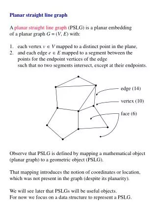
Planar straight line graph A planar straight line graph (PSLG) is a planar embedding of a planar graph G = (V, E) with: 1. each vertex vV mapped to a distinct point in the plane, 2. and each edge eE mapped to a segment between the points for the endpoint vertices of the edge such that no two segments intersect, except at their endpoints. edge (14) vertex (10) face (6) Observe that PSLG is defined by mapping a mathematical object (planar graph) to a geometric object (PSLG). That mapping introduces the notion of coordinates or location, which was not present in the graph (despite its planarity). We will see later that PSLGs will be useful objects. For now we focus on a data structure to represent a PSLG.
Doubly connected edge list (DCEL) The DCEL data structure represents a PSLG. It has one entry for each edge e in the PSLG. Each entry has 6 fields: V1 Origin of the edge V2 Terminus (destination) of the edge; implies an orientation F1 Face to the left of edge, relative to V1V2 orientation F2 Face to the right of edge, relative to V1V2 orientation P1 Index of entry for first edge encountered after edge V1V2, when proceeding counterclockwise around V1 P2 Index of entry for first edge after edge V1V2, when proceeding counterclockwise around V2 v3 f4 e3 f2 e5 v2 e1 v1 e4 f1 e2 f3 v4 Example (both PSLG and DCEL are partial)
2 2 3 F2 13 8 9 4 12 F6 11 1 3 10 F3 F1 F4 6 7 6 9 5 F5 1 4 7 8 5 Edge V1 V2 LeftF RightF PredE NextE ------------------------------------------------- 1 1 2 F6 F1 7 13 2 2 3F6F2 1 4 3 34F6 F3 2 5 4 3 9 F3 F2 3 12 5 4 6F5F3 8 11 6 6 7 F5 F4 5 10 7 1 5 F5 F6 9 8 8 45 F6 F5 3 7 9 1 7 F1 F5 1 6 10 7 8 F1 F4 9 12 11 6 9 F4 F3 6 4 12 9 8 F4 F2 11 13 13 2 8 F2 F1 2 10
Data structures If the PSLG has N vertices, M edges and F faces then we know N - M +F = 2 by Euler’s formula. DCEL can be described by six arrays: V1[1:M], V2[1:M], LeftF[1:M] Right[1:M], PredE[1:M] and NextE[1:M]. Since both the number of faces and edges are bounded by a linear function of N, we need O(N) storage for all these arrays. Define array HV[1:N] with one entry for each vertex; entry HV[i] denotes the minimum numbered edge that is incident on vertex vi and is the first row or edge index in the DCEL where vi is in V1 or V2 column. Thus for our example in the preceding slide HV=(1,1,2,3,7,5,6,10,4]. Similarly, define array HF[1:F] where F= M-N+2 , with one entry for each face; HF[i] is the minimum numbered edge of all the edges that make the face HF[i] and is the first row or edge index in the DCEL where Fii is in LeftF or RightF column. For our example, HF=(1,2,3,6,5,1). Both HV and HF can be filled in O(N) time each by scanning DCEL.
DCEL operations Procedure EdgesIncident use a DCEL to report the edges incident to a vertexvj in a PSLG. The edges incident to vj are given as indexes to the DCEL entries for those edges in array A [1: 3N-6] since M<= 3N-6. 1 procedure EdgesIncident(j) 2 begin 3 a = HV[j] /* Get first DCEL entry for vj, a is index. */ 4 a0 = a /* Save starting index. */ 5 A[1] = a 6 i = 2 /* i is index for A */ 7 if (V1[a] = j) then /* vertex j is the origin */ 8 a =PredE[a] /* Go on to next incident edge. */ 9 else /* vertex j is the destination vertex of edge a */ 10 a =NextE[a] /* Go on to next incident edge. */ 11 endif 12 while (aa0) do /* Back to starting edge? */ 13 A[i] = a 14 if (V1[a] = j) then 15 a = PredE[a] /* Go on to next incident edge. */ 16 else 17 a = NextE[a] /* Go on to next incident edge. */ 18 endif 19 i = i + 1 20 endwhile 21 end V2[a] NextE[a] a V1[a] PredE[a]
If we make the following changes, it will become a procedure • Faceincident[j] giving all the edges that constitute a face: • 3: a = HF[j] • And sustitute HV by HF and V1 by F1. • A will have a size A[1:N]. • Both EdgesIncident and Faceincident requires time proportional • to the number of incident edges reported. • How does that relate to N, the number of vertices in the PSLG? • We have these facts about planar graphs (and thus PSLGs): • (1) v - e + f = 2 Euler’s formula • (2) e 3v - 6 • (3) f 2/3e • (4) f 2v - 4 • where v = number of vertices = N • e = number of edges=M • f = number of faces=F • vO(N) by definition • eO(N) by (2) • EdgesIncident requires time O(N) and • DCEL requires storage O(N), one entry per edge.