Simetar Download
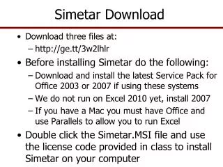
Simetar Download. Download three files at: http://ge.tt/3w2lhlr Before installing Simetar do the following: Download and install the latest Service Pack for Office 2003 or 2007 if using these systems We do not run on Excel 2010 yet, install 2007

Simetar Download
E N D
Presentation Transcript
Simetar Download • Download three files at: • http://ge.tt/3w2lhlr • Before installing Simetar do the following: • Download and install the latest Service Pack for Office 2003 or 2007 if using these systems • We do not run on Excel 2010 yet, install 2007 • If you have a Mac you must have Office and use Parallels to allow you to run Excel • Double click the Simetar.MSI file and use the license code provided in class to install Simetar on your computer
Multiple Regression Forecasts • Materials for this lecture • Demo Lecture 2 Multiple Regression.XLS • Read Chapter 15 Pages 8-9 • Read all of Chapter 16’s Section 13
Define Data Patterns • A time series is a chronological sequence of observations for a particular variable over fixed intervals of time • Daily • Weekly • Monthly • Quarterly • Annual • Six patterns for time series data (data we work with is time series data because use data generated over time). • Trend • Cycle • Seasonal variability • Structural variability • Irregular variability • Black Swans
Trend Variation • Trend a general up or down movement in the values of a time series over the historical period of observation • Most economic data contains at least one trend • Increasing, decreasing or flat trends • Trend represents long-term growth or decay • Trends caused by strong underlying forces, such as: • Technological changes • Change in tastes and preferences • Change in income and population • Market competition • Inflation and deflation • Policy changes
Cyclical Variation • Cycle is a recurring up and down movement around a trend • Cycles persist for 2 to 20 years from peak to peak • Business cycle is most notorious • Agriculture examples are cattle and hog cycles • Two components to a cycle • Expansion • Contraction • Cycles caused by • Changes in tastes and preferences • Economic activity (inflation and deflation) • Production cycles (animals) • Moon and sunspots? • Cycles vary in length and magnitude
Seasonal Variation • Periodic (cyclical) patterns in a time series that complete the cycle within a year • Caused by • Weather, seasons of the year • Production/marketing patterns • Customs and holidays • Agricultural production causes seasonal variation of prices • Holidays cause retail demand and sales to vary on a seasonal pattern • Thanksgiving – turkey • St. Patrick’s Day – corned beef and green beer • Easter – ham • Winter – cheese • Summer – ice cream and gasoline sales • Holidays and high temperatures – crushed ice
Structural Variation • Variables you want to forecast are often dependent on other variables Qt. Demand = f( Own Price, Competing Price, Income, Population, Season, Tastes & Preferences, Trend, etc.) Y = a + b (Time) • Structural models will explain most structural variation in a data series • Even when we build structural models, the forecast is not perfect • A residual remains as the unexplained portion
Irregular Variation • Erratic movements in time series that follow no recognizable regular pattern • Random, white noise, or stochastic movements • Risk is this non-systematic variability in the residuals • This risk leads to Monte Carlo simulation of the risk for our probabilistic forecasts • We recognize risks cannot be forecasted • Incorporate risks into probabilistic forecasts • Provide forecasts with confidence intervals
Black Swans (BSs) • BSs low probability events • An outlier “outside realm of reasonable expectations” • Carries an extreme impact • Human nature causes us to concoct explanations • Black swans are an example of uncertainty • Uncertainty is generated by unknown probability distributions • Risk is generated by known distributions • Recent recession was a BSs • A depression is a BSs • Dramatic increases of grain prices in 2006 and 2007 • Dramtaic increase in cotton price in 2010
Multiple Regression Forecasts • Structural model of the forecast variable is used when suggested by: • Economic theory • Knowledge of the industry • Relationship to other variables • Economic model is being developed • Examples of forecasting: • Planted acres – inputs sales businesses need this • Demand for a product – sales and production • Price of corn or cattle – feedlots, grain mills, etc. • Govt. payments – Congressional Budget Office • Exports or trade flows – international ag. business
Multiple Regression Forecasts • Structural model Ŷ = a + b1 X1 + b2 X2 + b3 X3 + b4 X4 + e Where Xi’s are exogenous variables that explain the variation of Y over the historical period • Estimate parameters (a, bi’s, and SEPe) using multiple regression (or OLS) • OLS is preferred because it minimizes the sum of squared residuals • This is the same as reducing the risk on Ŷ as much as possible, i.e., minimizing the risk for your forecast
Steps to Build Multiple Regression Models • Plot the Y variable in search of: trend, seasonal, cyclical and irregular variation • Plot Y vs. each X to see the structural relationship and how X may explain Y; calculate correlation coefficients to Y • Hypothesize the model equation(s) with all likely Xs to explain the Y, based on knowledge of model & theory • Forecasting wheat production, model is Plt Act = f(E(Pricet), Plt Act-1, E(PthCropt), Trend, Yieldt-1) Harvested Act = a + b Plt Act Yieldt = a + b Tt Prodt = Harvested Act * Yieldt • Estimate and re-estimate the model • Make the deterministic forecast • Make the forecast stochastic for a probabilistic forecast
US Planted Wheat Acreage Model Plt Act = f(E(Pricet), Yieldt-1, CRPt, Yearst) • Statistically significant betas for Trend (years variable) and Price • Leave CRP in model because of policy analysis and it has the correct sign • Use Trend (years) over Yieldt-1, Trend masks the effects of Yield
Multiple Regression Forecasts • Specify alternative values for X and forecast the Deterministic Component • Multiply Betas by their respective X’s • Forecast Acres for alternative Prices and CRP • Lagged Yield and Year are constant in scenarios
Multiple Regression Forecasts • Probabilistic forecast uses ŶT+I and SEP or Std Dev and assume a normal distrib. for residuals ỸT+i= ŶT+i + NORM(0, SEPT) or ỸT+i= NORM(ŶT+i , SEPT)
Multiple Regression Forecasts • Present probabilistic forecast as a PDF with 95% Confidence Interval shown here as the bars about the mean in a probability density function (PDF)
Growth Forecasts • Some data display a growth pattern • Easy to forecast with multiple regression • Add T2variable to capture the growth or decay of Y variable • Growth function Ŷ = a + b1T+ b2T2 Log(Ŷ) = a + b1 Log(T) Double Log Log(Ŷ) = a + b1 T Single Log See Decay Function worksheet for several examples for handling this problem
Multiple Regression Forecasts Single Log Form Log (Yt) = b0 + b1 T Double Log Form Log (Yt) = b0 + b1 Log (T)
Decay Function Forecasts • Some data display a decay pattern • Forecast them with multiple regression • Add an X variable to capture the growth or decay of forecast variable • Decay function Ŷ = a + b1(1/T) + b2(1/T2)
Forecasting Growth or Decay Patterns • Here is the regression result for estimating a decay function Ŷt = a + b1 (1/Tt) or Ŷt = a + b1 (1/Tt) + b2 (1/Tt2)
Multiple Regression Forecasts • Examine a structural regression model that contains Trend and an X variable Ŷ = a + b1T + b2Xtdoes not explain all of the variability, a seasonal or cyclical variability may be present, if so need to remove its effect
Goodness of Fit Measures • Models with high R2 may not forecast well • If add enough Xs can get high R2 • R-Bar2 is preferred as it is not affected by no. Xs • Selecting based on highest R2 same as using minimum Mean Squared Error MSE =(∑ et2)/T
Goodness of Fit Measures • R-Bar2 takes into account the effect of adding Xs where s2 is the unbiased estimator of the regression residuals and k represents the number of Xs in the model
Goodness of Fit Measures • Akaike Information Criterion (AIC) • Schwarz Information Criterion (SIC) • For T = 100 and k goes from 1 to 25 • The SIC affords the greatest penalty for just adding Xs. • The AIC is second best and the R2 would be the poorest.
Goodness of Fit Measures • Summary of goodness of fit measures • SIC, AIC, and S2 are sensitive to both k and T • The S2 is small and rises slowly as k/T increases • AIC and SIC rise faster as k/T increases • SIC is most sensitive to k/T increases
Goodness of Fit Measures • MSE works best to determine best model for “in sample” forecasting • R2 does not penalize for adding k’s • R-Bar2 is based on S2 so it provides some penalty as k increases • AIC is better then R2 but SIC results in the most parsimonious models (fewest k’s)

