Whole Genome Alignment: Techniques and Applications in Comparative Genomics
480 likes | 615 Vues
Whole Genome Alignment (WGA) involves the comparison of genomic DNA sequences of closely related organisms to infer evolutionary relationships and identify genetic differences. When aligning genomes, scientists must consider genome rearrangements and focus on syntenic regions to ensure accurate comparisons. This process helps uncover the evolutionary history of organisms, understand susceptibility to diseases, and identify potential drug targets. Various alignment strategies, including global and local algorithms, are employed based on the genetic context, enabling a comprehensive analysis of conserved and variable genomic regions.

Whole Genome Alignment: Techniques and Applications in Comparative Genomics
E N D
Presentation Transcript
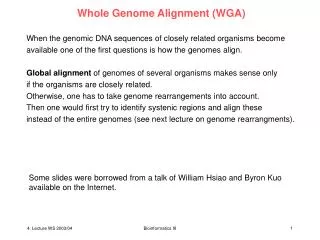
Whole Genome Alignment (WGA) When the genomic DNA sequences of closely related organisms become available one of the first questions is how the genomes align. Global alignment of genomes of several organisms makes sense only if the organisms are closely related. Otherwise, one has to take genome rearrangements into account. Then one would first try to identify systenic regions and align these instead of the entire genomes (see next lecture on genome rearrangments). Some slides were borrowed from a talk of William Hsiao and Byron Kuo available on the Internet. Bioinformatics III
Why align whole genome sequence? Biological Reasons Identify differences between organisms that may lead to the understanding of: • How the two organisms evolved? • E.g. How do we differ from chimps? • Why certain bacteria cause diseases while their cousins do not ? (Indels/ Mutations) • Why certain people are more susceptible to disease while others are not? (SNPs) – molecular medicine?? • Identifying new drug targets (targets are unique to pathogen) Bioinformatics III
Local- versus global-alignment algorithm strategies Top: Global alignments are generated when two DNA sequences (A and B) are compared and an optimal similarity score is determined over the entire length of the two sequences. Bottom: Local alignments are produced when two DNA sequences (A and B) are compared and optimal similarity scores are determined over numerous subregions along the length of the two sequences. The local-alignment algorithm works by first finding very short common segments between the input sequences (A and B), and then expanding out the matching regions as far as possible. Pennachio, Rubin, J Clin Invest. 111, 1099 (2003) Bioinformatics III
useful websites Pennachio, Rubin, J Clin Invest. 111, 1099 (2003) Bioinformatics III
Alignment strategies for different types of assemblies Couronne, ..., Dubchak, Genome Res. 13, 73 (2003) Bioinformatics III
Visualisation: Comparison of ApoE genomic sequence (a ) PipMaker analysis with human sequence in x and percentage similarity to chimpanzee in y. Exons are indicated by black boxes and repetitive elements by triangles above the plot. Each PIP horizontal bar indicates regions of similarity based on the percent identity of each gap-free segment in the alignment. Once a gap (insertion or deletion) is found within the alignment, a new bar is created to display the adjacent correspondent gap-free segment. (b) VISTA analysis with human sequence shown on x and percentage similarity to chimpanzee on y. The graphical plot is based on sliding-window analysis of the underlying genomic alignment. Blue and pink shading indicate conserved coding and noncoding DNA. Green and yellow bars immediately above the VISTA plot correspond to various repetitive DNA elements. (c ) PipMaker analysis with human sequence on x and percentage similarity to mouse on y. (d) VISTA analysis with human sequence on x and percentage similarity to mouse on y. Pennachio, Rubin, J Clin Invest. 111, 1099 (2003) Bioinformatics III
UCSC genome browser UCSC Genome Browser output for human/mouse sequence comparison of the ApoE gene (22). Human sequence is depicted on the x axis, and the numbering corresponds to the position of human chromosome 19 based on the UCSC June 2002 freeze (22). Note the different scoring system in contrast to percent identity, with peaks representing L-scores that take into account the context of the level of conservation. Conservation in relatively nonconserved regions receives higher L-scores than similar conservation in relatively highly conserved regions. As a second display of conservation, the "best mouse" track uses blocks whose length and shading represent the conservation. Pennachio, Rubin, J Clin Invest. 111, 1099 (2003) Bioinformatics III
local alignment: problem with repeats About 2% of the aligned base pairs of the human genome are covered by more than one mouse sequence fragment. In the example shown, several copies of the mouse pseudogene of Laminin B receptor (LAMR1) from different chromosomes were aligned to human LAMR1 (4th line from bottom). Couronne, ..., Dubchak, Genome Res. 13, 73 (2003) Bioinformatics III
sensitivity In the global human:mouse alignment more than one million regions are conserved at higher than 70% conservation at the 100-bp level – these regions cover > 200 Million bp. Only 62% of them are covered by base pairs of a (local) BLAT hit. This means that 38% of the conserved features are found only at the global alignment stage. Local alignment can therefore serve as anchoring system for a subsequent global alignment that will identify many additional conserved regions outside the anchors. Couronne, ..., Dubchak, Genome Res. 13, 73 (2003) Bioinformatics III
high sensitivity of global alignment Global alignment of the mouse finished sequence NT_002570 against the region found by BLAT anchors reveals conserved coding and non-coding elements not found by the BLAT program. The anchoring scheme is sensitive enough to provide the global alignment with the correct homology candidate. The location found for this mouse finished contig on the human genome, June 2002 (hg12/ncbi30) is chr20:42974590-42993423. Couronne, ..., Dubchak, Genome Res. 13, 73 (2003) Bioinformatics III
Specificity Specificity (how much of the alignment is correct?) is much more difficult to measure than sensitivity. One test: Measure coverage of human chromosome 20 by alignments of sequences from all mouse chromosomes except chromosome 2. (HC20 and MC2 are entirely syntenic.) Indeed, only a coverage of 6% is found for exons due, for example, of nonsystenic coverage coming from pseudogenes. Couronne, ..., Dubchak, Genome Res. 13, 73 (2003) Bioinformatics III
Specificity: Apolipoprotein(a) region Second test: The expressed gene apo(a) is only present in a subset of primates - most mammals lack apo(a). Shown are the coverage in this region by the mouse sequence utilizing Blastz and that obtained by Dubchak et al. Only the Dubchak method (see line „VISTA“) predicts that apo(a) has no homology in the mouse, as has been shown experimentally. Couronne, ..., Dubchak, Genome Res. 13, 73 (2003) Bioinformatics III
Additional information by global whole genome alignment • Difference in repeat patterns • Duplication (large fragment, chromosomal) • Tandem repeats • Large insertions and deletions • translocation (moving from one part of genome to another) • Single Nucleotide Polymorphism Bioinformatics III
Methods for WGA: iterative pairwise global alignment These Methods follow a general strategy of iteratively merging two multiple alignments of two disjoint subsets of sequences into a single multiple alignment of the union of those subsets. Construct a hash table on either the query string, or the database string (or both) for all possible substrings of a pre-specified size (say l) Find exactly matching substrings of length l using this hash table (seeds). In the second phase, these seeds are extended in both directions, and combined if possible, in order to find better alignments. If the global pairwise alignment of two genomic DNA sequences S1 and S2 is computed by standard dynamic programming algorithms (which requires O( | S1|∙| S2| time, where |S| is the length of sequence S) such iterative methods cannot be used in practice to align DNA sequences of entire genomes due to time and memory limitations. examples are: FASTA, BLAST, MegaBLAST, BL2SEQ, Wu-blast, flash,PipMaker (BLASTZ), and PatternHunter Bioinformatics III
Methods for WGA: anchor-based global multiple alignment These methods try to identify substrings of the sequences under consideration that they are likely parts of a global alignment. (As mentioned, these substrings can be obtained from local alignments). These substrings form „anchors“ in the sequences to be aligned. These methods first align the anchors and subsequently close the gaps (align the substrings between the anchors). Anchor-based alignment methods are well suited for aligning very long sequences. MUMmer is a very successful implementation of this strategy for aligning two genome sequences. other implementations: QUASAR, REPuter Bioinformatics III
What is MUMmer? • A.L. Delcher et al. 1999, 2002 Nucleic Acids Res. • http://www.tigr.org/tigr-scripts/CMR2/webmum/mumplot • Assume two sequences are closely-related (highly similar) • MUMmer can align two bacterial genomes in less than 1 minute • Use Suffix Tree to find Maximal Unique Matches • Maximal Unique Match (MUM) Definition: • A subsequence that occurs in two exactly matching copies, once in each input sequence, and that cannot be extended in either direction • Key idea: a significantly long MUM is certainly going to be part of the global alignment A maximal unique matching subsequence (MUM) of 39 nt (shown in uppercase) shared by Genome A and Genome B. Any extension of the MUM will result in a mismatch. By definition, an MUM does not occur anywhere else in either genome. Delcher et al. Nucleic Acids Res 27, 2369 (1999) Bioinformatics III
MUMmer: Key Steps • Locating MUMs (user-defined length) ACTGATTACGTGAACTGGATCCA ACTCTAGGTGAAGTGATCCA ACTGATTACGTGAACTGGATCCA ACTCTAGGTGAAGTGATCCA 10 1 20 ACTGATTACGTGAACTGGATCCA ACTC--TAGGTGAAGTG-ATCCA 1 10 20 Bioinformatics III
Definition of MUMmers • For two strings S1 and S2 and a parameter l • The substring u is an MUM sequence if: • |u| > l • u occurs exactly once in S1 and it occurs exactly once in S2 (uniqueness) • For any character a neither ua nor au occurs both in S1 and in S2 (maximality) Bioinformatics III
How to find MUMs? • Naïve Approach • Compare all subsequences of genome A with all subsequences of genome B O(nn) • Suffix Tree • Naïve approach to build a suffix tree • Quadratic time, space • McCreight’s algorithm • Linear time, linear space • Clever use of pointers Bioinformatics III
Suffix Tree • Suffix trees are well-established since > 20 years. • Some properties: • a “suffix” starts at any position I of the sequence and goes until its end. • sequence of length N string has N suffixes • N leaves • Each internal node has at least 2 child nodes • No 2 edges out of the same node can have edge beginning with the same character • add $ to the end CACATAG$ Bioinformatics III
Constructing a Suffix Tree CACATAG$ Suffixes: 1. CACATAG$ C A C A T A G $ 1 Bioinformatics III
Constructing a Suffix Tree CACATAG$ A Suffixes: 1. CACATAG$ 2. ACATAG$ C A C C A A T T A A G G $ $ 2 1 Bioinformatics III
Constructing a Suffix Tree CACATAG$ A Suffixes: 1. CACATAG$ 2. ACATAG$ 3. CATAG$ C A C C A A T T T A A A G G G $ $ $ 2 3 1 Bioinformatics III
Constructing a Suffix Tree CACATAG$ A Suffixes: 1. CACATAG$ 2. ACATAG$ 3. CATAG$ 4. ATAG$ C T A G $ 4 A C C A A T T T A A A G G G $ $ $ 2 3 1 Bioinformatics III
Constructing a Suffix Tree CACATAG$ A Suffixes: 1. CACATAG$ 2. ACATAG$ 3. CATAG$ 4. ATAG$ 5. TAG$ C T A G $ 4 A C C T A A T T A T A A A G G G G $ $ $ $ 2 3 1 5 Bioinformatics III
Constructing a Suffix Tree CACATAG$ A Suffixes: 1. CACATAG$ 2. ACATAG$ 3. CATAG$ 4. ATAG$ 5. TAG$ 6. AG$ C T A G $ 4 A C C T A A T G T A T $ A A A G 6 G G G $ $ $ $ 2 3 1 5 Bioinformatics III
Constructing a Suffix Tree CACATAG$ G $ 7 A Suffixes: 1. CACATAG$ 2. ACATAG$ 3. CATAG$ 4. ATAG$ 5. TAG$ 6. AG$ 7. G$ C T A G $ 4 A C C T A A T G T A T $ A A A G 6 G G G $ $ $ $ 2 3 1 5 Bioinformatics III
Constructing a Suffix Tree CACATAG$ $ G $ 8 7 A Suffixes: 1. CACATAG$ 2. ACATAG$ 3. CATAG$ 4. ATAG$ 5. TAG$ 6. AG$ 7. G$ 8. $ C T A G $ 4 A C C T A A T G T A T $ A A A G 6 G G G $ $ $ $ 2 3 1 5 Bioinformatics III
Saving Space CACATAG$ [8, 1] [7, 2] [2, 1] Suffix trees can become very large because they are of size comparable to the genome. Saving space (memory) is therefore crucial. [5, 4] [1, 2] [7, 2] [3, 6] [5, 4] [3, 6] [5, 4] Bioinformatics III
Searching a Suffix Tree $ G $ Search Pattern: CATA 8 7 A C T A G $ 4 A C C T A A T G T A T $ A A A G 6 G G G $ $ $ $ 2 3 1 5 Bioinformatics III
Searching a Suffix Tree $ G $ Search Pattern: ATCG 8 7 A C T A G $ 4 A C C T A A T G T A T $ A A A G 6 G G G $ $ $ $ 2 3 1 5 Bioinformatics III
MUMmer 1.0: How to find MUMs? • Build a suffix tree from all suffixes of genome A • Insert every suffix of genome B into the suffix tree • Label each leaf node with the genome it represents Bioinformatics III
How MUMmer 1.0 finds MUMs? • Unique Match: • internal node with 2 child nodes where the leaf nodes are from different genomes! • Unique matches may not be maximal • Maximal matches can be found by investigating the unique match furthest away from the root node • User specifies the minimum length of MUMs to be identified T $ A C A, 4 A T C A # A $ T A # # $ B, 4 B, 3 A, 3 A, 2 B, 2 A T $ # A, 1 B, 1 Genome A: ACAt$ Genome B: ACAa# Bioinformatics III
Sorting the MUMs • MUMs are sorted according to their positions in genome A • Use a variation of Longest Increasing Subsequence (LIS) to find sequences in ascending order in both genomes • Takes into account lengths of sequences represented by MUMs, and overlaps • O(klogk) running time, k = number of MUMs Genome A: 3 1 2 4 5 6 7 Genome B: 3 6 5 1 2 4 7 Genome A: 1 2 4 6 7 Genome B: 6 7 2 1 4 Each MUM is indicated only by a number, regardless of its length. Top alignment shows all MUMs. The shift of MUM 5 in Genome B indicates a transposition. The shift of MUM 3 could be simply a random match or part of an inexact repeat sequence. Bottom alignment shows just LIS of MUMs in Genome B. Bioinformatics III
4 types of gaps in MUM alignment These examples are drawn from the alignment of the two M.tuberculosis genomes. Delcher et al. Nucleic Acids Res 27, 2369 (1999) Bioinformatics III
Closing the Gaps • SNP • Simple case: gap of one base between adjacent MUMs • when adjacent to repeat sequences: treated as tandem repeats • Variable / Polymorphic Region • Small region: dynamic programming alignment • Large region: recursively apply MUMmer with reduced minimum cut-off length • Insertions / Deletion • Transposition: out of alignment order • Simple insertion: not in the alignment • Repeats • Tandem repeats are detected by overlapping MUMs • Other repeats (i.e. duplication) are treated as gaps Close gaps by performing local alignment on portion between the aligned MUMs (using e.g. Smith-Waterman). Bioinformatics III
some positions are not uniquely defined Repeat sequences surrounded by unique sequences. For the purposes of illustration, other characters besides the four DNA nucleotides are used. Delcher et al. Nucleic Acids Res 27, 2369 (1999) Bioinformatics III
example: Alignment of 2 M.tuberculosis strains CDC1551 H37Rv Global alignment of two very similar tubercolosis strains: Single green lines in the center connect single-base differences between the genomes. Blue v-shaped lines indicate insertions. The first two v-shaped insertions are large insertions in H37Rv, and the third insertion is a very small insertion in CDC1551. This last insertion appears as a line rather than a v-shape due to the resolution of the displayed region. The genes from both genomes are displayed as arrows, with color-coding to indicate the role assigned to each gene. Note that both of the large insertions shown here contain genes. White lines (gaps) appearing in the middle of some arrows indicate silent mutations in those genes. Delcher et al. Nucleic Acids Res 27, 2369 (1999) Bioinformatics III
Example: alignment of 2 micoorganisms The genome of M.genitalium is only ca. 2/3 the size of M.pneumoniae. Alignment of M.genitalium and M.pneumoniae using FASTA (top), 25mers (middle) and MUMs (bottom). In all three plots, a point indicates a `match' between the genomes. In the FASTA plot a point corresponds to similar genes. In the 25mer plot, each point indicates a 25-base sequence that occurs exactly once in each genome. In the MUM plot, points correspond to MUMs as defined in the main text: 5 translocations can be seen. Delcher et al. Nucleic Acids Res 27, 2369 (1999) Bioinformatics III
Example: alignment human:mouse Alignment of even more distant species: human and mouse. Here: alignment of a 222 930 bp subsequence of human chromosome 12p13, accession no. U47924, to a 227 538 bp subsequence of mouse chromosome 6, accession no. AC002397. Each point in the plot corresponds to an MUM of [ge]15 bp. Delcher et al. Nucleic Acids Res 27, 2369 (1999) Bioinformatics III
MUMmer 2.0: Improvements • Memory Requirement • Reduced memory usage per base from 37 bytes to 20 bytes • Finding Initial Exact Matches • Store only one sequence as suffix tree • Suffixes of second sequence are streamed against the tree • Saves 1/2 of memory usage • Ability to align protein sequences • Whole Genome Alignments can now be done on 100 Mb genomes within minutes or less Bioinformatics III
Query suffix tree A sample suffix tree showing the streaming behavior for finding matches between a query and a reference. Delcher et al. Nucleic Acids Res 30, 2478 (2002) Bioinformatics III
Current disadvantages linear space still means huge memory requirement for medium size genomes – e.g. 100mb genome => ~4Gb of working memory - Repeats are not handled specifically - tandem repeats as overlapping MUMs - duplications are ignored - Smith-Waterman DP used to fill in small gaps; large gaps ignored - not efficient for aligning distantly related genomes which have few MUMs and many gaps Bioinformatics III
Conclusion • Suffix tree methodology meant a major breakthrough in full genome alignment algorithm • MUMmer 2 made some improvements in time and space requirements • possible to improve the data structure further – e.g. by using suffix array instead of suffix tree • Apply to Multiple Genome Alignment (implemented in MGA) Bioinformatics III
MGA MGA is a very promising anchor-based method that allow to align 3 genomes. In the first phase, all maximal multiple exact matches (multiMEMs) are detected whose length exceeds a given threshold. A multiMEMs occurs in all genomes to be aligned and cannot simultaneously be extended to the left or right in every genome. O(kn + r) where k is the number of genomes, n is their total length, and r is the number of right maximal multiple exact matches. In the second phase, MGA computes the „anchors“, consisting of the longest non-overlapping sequence of multiMEMs that occur in the same order in each of the genomes. O(k·m2) where m is the number of multiMEMs. In the third phase, MGA closes the gaps between the anchors by recursively applying the same method a certain number of times, thereby lowering the length threshold for the multiMEMs. Remaining gaps: short gaps are closed by multiple sequence alignment with ClustalW. Long gaps remain unaligned in order to cope with long insertions, deletions etc. Höhl, Kurtz, Ohlebusch, Bioinformatics 18, S312 (2002) Bioinformatics III