PSI-BLAST: Sequence Alignment Lecture 8

1. C E N T E R F O R I N T E G R A T I V E B I O I N F O R M A T I C S V U Master Course Sequence Alignment Lecture 8Database searching (2)

2. PSI-BLAST • Position-Specific Iterated BLAST • A profile (called PSSM by BLAST – Position Specific Scoring Matrix) is derived from the result of the first search (using a single query sequence) • Database is searched against the profile (instead of a sequence) in subsequent rounds • Up to 3-10 iterations are recommended

3. PSI-BLAST steps in words • Query sequences are first scanned for the presence of so-called low-complexity regions (Wooton and Federhen, 1996), i.e. regions with a biased composition likely to lead to spurious hits; are excluded from alignment. • The program then initially operates on a single query sequence by performing a gapped BLAST search • Then, the program takes significant local alignments (hits) found, constructs a multiple alignment (master-slave alignment) and abstracts a position-specific scoring matrix (PSSM) from this alignment. • The database is rescanned in a subsequent round, now using the PSSM, to find more homologous sequences. Iteration continues until user decides to stop or the search has converged

4. Profile • a Profile is a generalized form of sequence • probabilities instead of a letter A C D    W Y 0.5 0 0 . .  0 0.5 0.3 0.1 0 . .  0.3 0.3 0.2 0.0 0.1 . .  0.4 0.3 ... ... ... ... ... ... ... ... 0 0.5 0.2 . .  0.1 0.2

5. Constructing a profile • Take significant BLAST hits • Make an alignment • Assign weights to sequences • Construct profile A C D    W Y 0.5 0 0 . .  0 0.5 0.3 0.1 0 . .  0.3 0.3 0 0.5 0.2 . .  0.1 0.2 0.2 0.0 0.1 . .  0.4 0.3 ... ... ... ... ... ... ... ...

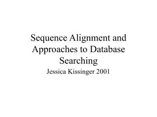
6. PSI BLAST:Constructing the Profile Matrix Figure from: Altschul et al. Nucleic Acids Research 25, 1997

7. Profile calculation example using frequency normalisation and log conversion (A) 12345 S1 GCTCC S2 AATCG S3 TACGC S4 GTGTT S5 GTAAA S6 CGTCC Normalise by dividing by overall frequencies Convert to log to base of 2 profile Sum corresponding log odds matrix scores (B) Match GATCA to PSSM Score = 1.11 + 0.72 + 0.89 + 0.74 - 0.23 = 3.23 Find nucleotides at corresponding positions

8. PSI BLAST: Determining profile elements more reliably using pseudo-counts • the value for a given element of the profile matrix is given by: • where the probability of seeing amino acid aiin column j is estimated as: Overall alignment frequency (preceding slide) e.g.  = number of sequences in profile, =1 Observed frequency Pseudocount (e.g. database frequency)

9. PSI BLAST: Determining profile elements more reliably using pseudo-counts • Pseudo-counts: • mix observed a.a. frequencies with prior (e.g. database) frequencies • drawback is pulling all frequencies to prior frequencies, which reduces the differences between sequences • are useful when multiple alignment contains only few sequences so that there is no statistical sample per column yet • with greater numbers of sequences in the MSA, the profile becomes less dependent on priors

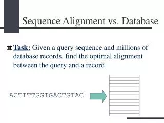
10. PSI-BLAST iteration graphic… Query sequence Q xxxxxxxxxxxxxxxxx Gapped BLAST search Query sequence Q Low-complexity region xxxxxxxxxxxxxxxxx Database hits A C D . . Y iterate PSSM Gapped BLAST search PSSM A C D . . Y Database hits

11. Another PSI-BLAST iteration graphic… Run query sequence against database Q Run PSSM against database hits T DB PSSM Discarded sequences

12. (A) (B) (C) (D) Figure 6

13. PSI-BLAST entry page Paste your query sequence Switch this off for default run

15. 1 - This portion of each description links to the sequence record for a particular hit. 2 - Score or bit score is a value calculated from the number of gaps and substitutions associated with each aligned sequence. The higher the score, the more significant the alignment. Each score links to the corresponding pairwise alignment between query sequence and hit sequence (also referred to as subject sequence). 3 - E Value (Expect Value) describes the likelihood that a sequence with a similar score will occur in the database by chance. The smaller the E Value, the more significant the alignment. For example, the first alignment has a very low E value of e-117 meaning that a sequence with a similar score is very unlikely to occur simply by chance. 4 - These links provide the user with direct access from BLAST results to related entries in other databases. ‘L’ links to LocusLink records and ‘S’ links to structure records in NCBI's Molecular Modeling DataBase.

16. ‘X’ residues denote low-complexity sequence fragments that are ignored

17. PHI-BLAST (Pattern Hit Initiated) • Method to find database sequences based on a given sequence pattern • Sequence patterns are found using regular expressions (comes later in this course) in PROSITE format (PROSITE is a database of functional sequence motifs expressed as regular expressions or profiles) • Occurrences need not exceed threshold T • Extension and alignment are the same as in Gapped (or PSI-) Blast • Scoring scheme is different (stricter) due to the importance of pattern occurrence

18. FASTA • First homology searching method (FASTP – Lipman & Pearson, 1985) • Until gapped-BLAST and PSI-BLAST appeared (1997), FASTA has been the better method • Compares a given query sequence with a library of sequences and calculates for each pair the highest scoring local alignment • Speed is obtained by delaying application of the dynamic programming technique to the moment where the most similar segments are already identified by faster and less sensitive techniques • FASTA routine operates in four steps:

19. FASTA • Operates in four steps: • Rapid searches for identical words of a user specified length occurring in query and database sequence(s) (Wilbur and Lipman, 1983, 1984). For each target sequence the 10 regions with highest density of ungapped common words are determined. • These 10 regions are rescored using Dayhoff PAM-250 residue exchange matrix (Dayhoff et al., 1983) and the best scoring region of the 10 is reported under init1 in the FASTA output. • Regions scoring higher than a threshold value Tand being sufficiently near each other in the sequence are joined, now allowing gaps. The highest score of these new fragments can be found under initn in the FASTA output. T is set such that only a small fraction of database sequences are retained. These are the only ones that are reported to the user. Until here things are quick!

20. FASTA • Operates in four steps (continued): • full dynamic programming alignment (Chao et al., 1992) over the final region which is widened by 32 residues at either side, of which the score is written under opt in the FASTA output. This is slow – O(n2)

21. FASTA output example DE METAL RESISTANCE PROTEIN YCF1 (YEAST CADMIUM FACTOR 1). . . . SCORES Init1: 161 Initn: 161 Opt: 162 z-score: 229.5 E(): 3.4e-06 Smith-Waterman score: 162; 35.1% identity in 57 aa overlap 10 20 30 test.seq MQRSPLEKASVVSKLFFSWTRPILRKGYRQRLE :| :|::| |:::||:|||::|: | YCFI_YEAST CASILLLEALPKKPLMPHQHIHQTLTRRKPNPYDSANIFSRITFSWMSGLMKTGYEKYLV 180 190 200 210 220 230 40 50 60 test.seq LSDIYQIPSVDSADNLSEKLEREWDRE :|:|::| |:::||:|||::|: | YCFI_YEAST EADLYKLPRNFSSEELSQKLEKNWENELKQKSNPSLSWAICRTFGSKMLLAAFFKAIHDV 240 250 260 270 280 290

22. FASTA • (1) Rapid identical word searches: • Searching for k-tuples of a certain size within a specified bandwidth along search matrix diagonals. • For not-too-distant sequences (> 35% residue identity), little sensitivity is lost while speed is greatly increased. • Technique employed is known as hash coding or hashing: a lookup table is constructed for all words in the query sequence, which is then used to compare all encountered words in each database sequence.

23. HASHING (general) • rapid identical word searches • a lookup table is constructed for all words in the query sequence, which is then used to compare all encountered words in each database sequence • Example of hashing: the telephone book to find persons’ phone numbers (names are ordered) • you do not need to search through all names until you find the person you want • In computer speak: find a function f such that f(name) can be directly assigned to address in computer, where the telephone number is stored

24. HASHING (cont.) This takes too long…… .. 0044 20 84453759 0044 20 84457643 0044 51 27655423 ‘Jones, D.A.’ ‘Mill, J.’ ‘Anson,F.P.L’

25. HASHING (cont.) Hash array Name = ‘Jones’ F(‘Jones’) 0044 20 84453759 • For sequences: • name is subword in database sequence • telephone number is sequence position(s) of subword

26. HASHING (cont.) Hash array Name = ‘Jones’ F(‘Jones’) .. 0044 20 84453759 ‘Jones, D.A.’ clashes • Hash function should avoid clashes: • clashes take more time • but need less memory for hash array

27. HASHING (cont.) Example of hash function: Take position of letter in alphabet (p(a)=1, p(b)=2, p(c)=3,..) F(‘Jones’) = p(J)+p(o)+p(n)+p(e)+p(s) = 10+15+14+5+19=63 So, ‘Jones’ goes to slot 63 in Hash array What do you think about this function? Will there be clashes?

28. HASHING in FASTASequence positions in query are hashed Query: ERLFERLAC ……… DB: MERIFERLAC ……… Query hash table: Word Position ER 1, 5 RL 2, 6 LF 3 FE 4 LA 7 AC 8 …. … You only need to go through the DB sequence once: for each word encountered (ME, ER, RI, IF, ..), check the query hash list for the word. If found, you immediately have the query sequence positions of the word. You also know the position you are at in the DB sequence, and so you can fill in the m*n matrix with diagonals (see earlier slide step 1). Algorithmic speed therefore is linear with (DB) sequence length or O(n). Compare this to finding all word match positions without a hash list (complexity is O(m*n)).

29. 0 1 … 74 …. 83 …. 180 … 184 … 289 … 8 … 1 … 4 … 7 … 3 … 2 … 1 2 3 4 5 6 7 89 5 6 0 0 0 0 0 0 0 Query: ERLFERLAC 123456789 One-let codes: ACDEFGHIKLMNPQRSTVWY 0 5 10 15 Query hash table: Word Hash Position ER 3*20+14 1, 5 RL 14*20+9 2, 6 LF 9*20+4 3 FE 4*20+3 4 LA 9*20+0 7 AC 0*20+1 8 E=3, R=14 h(‘ER’)=320+14 Hash array Chaining array DB: MERIFERLAC

30. FASTA • The k-tuple length (step 1) is user-defined and is usually 1 or 2 for protein sequences (i.e. either the positions of each of the individual 20 amino acids or the positions of each of the 400 possible dipeptides are located). • For nucleic acid sequences, the k-tuple is 5-20 (often 11), and should be longer because short k-tuples are much more common due to the 4 letter alphabet of nucleic acids. The larger the k-tuple chosen, the more rapid but less thorough, a database search.

31. Scoring BLAST alignments • Score should optimise the chance to select proper hits (True Positives) • Scoring alignments is dependent on • The scoring system used (residue exchange matrix and gap penalty regime) • Characteristics of the sequence database (size, residue composition) • The BLAST way of scoring has been adopted by other methods as well; e.g., some implementations of FASTA, etc.

32. Alignment Bit Score B = (S – ln K) / ln 2 • S is the raw alignment score • The bit score (‘bits’) B has a standard set of units • The bit score B is calculated from the number of gaps and substitutions associated with each aligned sequence. The higher the score, the more significant the alignment • and K and are statistical parameters associated with a given scoring system (e.g. BLOSUM62 in Blast) • See Altschul and Gish, 1996, for a collection of values for  and K over a set of widely used scoring matrices. • Because bit scores are normalized with respect to the scoring system, they can be used to compare alignment scores from different searches based on different scoring schemes (a.a. exchange matrices)

33. What is the statistical significance of an alignment • To get a null model: extract local alignments from random sequences • P-value • The probability of obtaining the result bypure chance • An alignment giving a lower P-value than a threshold value set by the user is considered a hit.

34. Normalised sequence similarity The p-valueis defined as theprobability of seeing at least one unrelated score S greater than or equal to a given score x in a database search over n sequences. This probability follows the Poisson distribution (Waterman and Vingron, 1994): P(x, n) = 1 – e-nP(S x), where n is the number of sequences in the database Depending on x and n (fixed)

35. E-value • The concept of P-value applies to single comparisons • What with searching in a large database? Task. Having a protein, we want to find similar ones in a large database (4 mln sequences in NR DB). We are interested in P-value < 0.01Count the number of hits we’ll get by chance alone.

36. Normalised sequence similarityStatistical significance The E-value is defined as the expected number of non-homologous sequences with score greater than or equal to a score x in a database of n sequences: E(x, n) = nP(S x) For example, if E-value = 0.01, then the expected number of random hits with score Sx is 0.01, which means that this E-value is expected by chance only once in 100 independent searches over the database. if the E-value of a hit is 5, then five fortuitous hits with S x are expected within a single database search, which renders the hit not significant.

37. A model for database searching score probabilities • Scores resulting from searching with a query sequence against a database follow the Extreme Value Distribution (EVD) (Gumbel, 1955). • Using the EVD, the raw alignment scores are converted to a statistical score (E value) that keeps track of the database amino acid composition and the scoring scheme (a.a. exchange matrix)

38. Extreme Value Distribution y = 1 – exp(-e-(x-)) Probability density function for the extreme value distribution resulting from parameter values  = 0 and  = 1, [y = 1 – exp(-e-x)], where  is the characteristic value (where the EVD peaks) and  is the decay constant.

39. Extreme Value Distribution (EVD) EDV approximation real data You know that an optimal alignment of two sequences is selected out of many suboptimal alignments, and that a database search is also about selecting the best alignment(s). This bodes well with the EDV which has a right tail that falls off more slowly than the left tail. Compared to using the normal distribution, when using the EDV an alignment has to score further away from the expected mean value to become a significant hit.

40. Extreme Value Distribution The probability of a score S to be larger than a given value x can be calculated following the EDV as: E-value: P(S x) = 1 – exp(-e -(x-)), where  =(ln Kmn)/, and K a constant that can be estimated from the background amino acid distribution and scoring matrix (see Altschul and Gish, 1996, for a collection of values for  and K over a set of widely used scoring matrices).

41. Extreme Value Distribution Using the equation for  (preceding slide), the probability for the raw alignment score S becomes P(S x) = 1 – exp(-Kmne-x). In practice, the probability P(Sx) is estimated using the approximation 1 – exp(-e-x) e-x, which is valid for large values of x. This leads to a simplification of the equation for P(Sx): P(S  x)  e-(x-) = Kmne-x. The lower the probability (E value) for a given threshold value x, the more significant the score S.

42. Normalised sequence similarityStatistical significance • Database searching is commonly performed using an E-value in between 0.1 and 0.001. • Low E-values decrease the number of false positives in a database search, but increase the number of false negatives, thereby lowering the sensitivity of the search.

43. Words of Encouragement • “There are three kinds of lies: lies, damned lies, and statistics” – Benjamin Disraeli • “Statistics in the hands of an engineer are like a lamppost to a drunk – they’re used more for support than illumination” • “Then there is the man who drowned crossing a stream with an average depth of six inches.” – W.I.E. Gates