Download
1 / 29
290 likes | 548 Vues
Albert-Jan Boonstra Mark Bentum Mathheijs Eikelboom. LOFAR RFI Mitigation spatial filtering at station level. Contents. LOFAR overview Spectrum environment RFI mitigation in LOFAR Data model, spatial filtering algorithm Spatial filtering in LOFAR, considerations Spatial filter results

E N D
Albert-Jan Boonstra Mark Bentum Mathheijs Eikelboom LOFAR RFI Mitigationspatial filtering at station level RFI2010 Workshop, Groningen, Nl, March 29-31, 2010
RFI2010 Workshop, Groningen, Nl, March 29-31, 2010 Contents • LOFAR overview • Spectrum environment • RFI mitigation in LOFAR • Data model, spatial filtering algorithm • Spatial filtering in LOFAR, considerations • Spatial filter results • Conclusion
RFI2010 Workshop, Groningen, Nl, March 29-31, 2010 LOFAR signal processing, overview Low Band Antenna High Band Antenna HBA antenna beam LBA receiver RSP 1 x 32 MHz station beams BlueGene central Processor CEP (correlator) synth. beams LOFAR: fsky ~ 30 – 240 MHz
RFI2010 Workshop, Groningen, Nl, March 29-31, 2010 LOFAR CS1 configuration 2006-2008 – Exloo Exloo R.Nijboer 2006 LBA antenna layout LBA CS10 • Operational Oktober 1, 2006 with “final” prototype hardware at Exloo • 96 dual-dipole LBA antennas distributed over ~500m: • one cluster with 48 dipoles • three clusters of 16 dipoles Total 24 microstation, 4 dipoles each Goal: emulate LOFAR with 24 micro-stations at reduced bandwidth or act as a single station at full BW
RFI2010 Workshop, Groningen, Nl, March 29-31, 2010 LOFAR status Stations 18 core stations + 18 remote stations + 8 int. Validated: 14 CR, 6 RS In progress: 6 CS, 1 RS, 3 German, 1 French Next: 9 RS, 1 UK, 1 Germany, 1 Sweden
RFI2010 Workshop, Groningen, Nl, March 29-31, 2010 LOFAR numbers Number of sensors on the various fields: Core station fields (18) 96 Low Band Antennas, 2 x 24 High Band Antenna Tiles (HBA field is split) Remote station fields (18) 96 Low Band Antennas, 48 High Band Antenna Tiles Microbaromater (infrasound) Geo-Remote station fields (10) Geophones & Microbarometers International station fields (8) 96 Low Band Antennas, 96 High Band Antenna Tiles Numbers for the LOFAR telescope performance Frequency range: 30- 80 MHz and 120 - 240 MHz Polarisations 2 Bandwidth 32 MHz (currently 48 MHz investigated) Stations: 18 core, 18 remote, 8 international Baseline length: 100 m to 1500 km Simult. dig. beams: 8 Sample bit depth: 12 Spectral resolution: 0.76 kHz
RFI2010 Workshop, Groningen, Nl, March 29-31, 2010 Some LOFAR imaging results 2007 2004 2006 2007 LOFAR all-sky image Stefan WIjnholds 25 June 2006 LOFAR HBA tile all-sky image Michiel Brentjens, 22 nov. 2007 LOFAR LBA alll-sky image Sarod Yatawatta & Jan Noordam 20 April 2007 2008 2008 2010 2009 LOFAR all-sky image Stefan Wijnholds 19 Nov. 2008 High-resolution LOFAR 3C61.1 image Credit: Reinout van Weeren (Sterrewacht Leiden) 8 feb 2010 Deep LOFAR HBA Image Sarod Yatawatta, 21 Feb. 2008 Cas A, Sarod Yatawatta 23 Dec. 2009
RFI2010 Workshop, Groningen, Nl, March 29-31, 2010 Spectrum environment Spectrograms 2009 TV band I land mobile land mobile FM band II AM RAS Lopik land mobile mobile frequency (MHz) frequency (MHz) RAS TV#6,7,... DAB aviation ambu- lance, taxi FM band II geostat. mil. satellite pager TV band III / DAB (DVB) mariphone weather sat.
RFI2010 Workshop, Groningen, Nl, March 29-31, 2010 LOFAR overview spectral estimation: derive for AM from R LOFAR station on-line correlator One covariance matrix R per second 512 subbands correlated in ~8.5 min. R Spatial filtering: wnew = P w spectral estimation: multiply one arm per interferometer with: eit Rclean = R-R
RFI2010 Workshop, Groningen, Nl, March 29-31, 2010 The radio spectrum: occurrence of weak RFI Tsky = 333 K Nf = 256 Nt = 300 = 60 s t = 5 h f = 0.76 kHz LOFAR High Band Antenna var(R11) = 4 / N 1 minute: ~ 0.02 dB relatively few weak RFI sources: “horizon effect”
RFI2010 Workshop, Groningen, Nl, March 29-31, 2010 The radio spectrum: effect on data transport rate • Purpose: • - increase the number of beams from 8 to 24 (both for 24 MHz bw) • - Without increase of station output data rate • Solution: reduce data rate to the LOFAR central processor from 16 to 4 bits (complex) for each beam Loss when using 4 bit could be solved by spatial filters at stations, but only for fixed transmitters (“fast moving nulls” would hamper calibration) Experiments in cleanest part of the spectrum indicated that < 10% of the data would be lost (no spatial filtering applied). e.g. L2007-0189525 HBA bands: In 3 of 23 bands: loss @ 16 bits: 0% @ 4 bits ~ 50% In 20 of 23 bands: no loss Average loss: 6.5%
RFI2010 Workshop, Groningen, Nl, March 29-31, 2010 Requirement: “smooth” station beamshape changes • LOFAR CS1 calibration/imaging • Observation: • 16 single-dipole stations, 48 h • 20 subbands, each 0.14 MHz “Calibrated”: removing phase drift (uv) “Residual”: peeling CasA and CygA Credit: Sarod Yatawatta, ASTRON • LOFAR ITS 2004 observations • 60 antennas, 26.75 MHz, basel.<200 m • with transmitter (left) • after subtraction filtering (right) • after projection filtering (middle) • LOFAR spatial filtering • At stations, filters for fixed directions (at subband level, ~ 200 kHz) • Post correlation: offline spatial filtering (in ~1 kHz channels)
RFI2010 Workshop, Groningen, Nl, March 29-31, 2010 t t Data model – signal model Consider an array of p antennas with baselines : bij = ri-rj Array output signals xi(t) and the noise signals ni(t) (from LNAs, spillover etc) are stacked in a vector: x(t) = [x1(t), … , xp(t)]t, n(t) = [n1(t), … , np(t)]t Suppose there is one source (astronomical or RFI) with signal s(t) from direction s, and with spatial signature vector a: The signal vector is defined by: x(t) = a s(t) + n(t)
RFI2010 Workshop, Groningen, Nl, March 29-31, 2010 Data model – covariance model Define the signal covariance sample estimate (observational data): R = xnxnH with xn = x (nTs) Given i.i.d. noise vector n(t), E{n(t)n(t)H} = n2I, and E{s(t)}2 = 2: R = E{R} = 2aaH + n2I Data model easily exended to multiple sky sources and multiple RFI sources Complication: low frequency sky contains strong extended structures Solution: extend model, use baseline restrictions, factor analysis algorithms However: this is not always a problem, e.g. in estimating DOA of strong RFI N n=1 ^ ^
RFI2010 Workshop, Groningen, Nl, March 29-31, 2010 Spatial filtering after correlation Data model with sky sources having covariance Rv, and interference with power r2 and signature vector ar: R = Rv + n2I + rararH Spatial filtering using projections Projection matrix: P = I – ar (arHar) -1arH note: Par = 0, Pa ≠0 Applying projection: R = P R P Spatial filtering using subtraction: R = R – r2ararH Note: the subtraction filter can be rewritten as a projection filter by adding a scaling factor , dependent on the noise and on the RFI power: P = I – ar (arHar)-1arH cf. A. Leshem, A.J. van der Veen, and A.J. Boonstra. Multichannel interference mitigation techniques in radio astronomy. The Astrophysical Journal Supplement Series, 131(1):355–373, November 2000. ~ ^ ~ ^
RFI2010 Workshop, Groningen, Nl, March 29-31, 2010 Beamforming and spatial filtering beamfomer output y=wHx to central processor (BlueGene) local processing: station correlator, one second integrated R every 512 seconds- used for station calibration and RFI mitigation narrow band beamforming x1 w1 x2 w2 Source power:IB = Ryy = E{yyH} = wHE{xxH}w = wHRw => station sky map Ib(s) y = wHx … Recall data model: R = s2aaH + n2 I Maximum if w = a: wHRw = s2wHa aHw + n2wHw xp wp Spatial filtering (beamformer impl.), with P a spatial filter: w’ = P w And: IB = wH PRP w
RFI2010 Workshop, Groningen, Nl, March 29-31, 2010 How to find DOA and time-occupancy • DOA: • From a subspace analysis, R =U U: • Finding maxima in sky maps • Transmitter locations may be known • Using factor analysis, efficient rank-one methods ITS data Credit: M.Tanigawa& M.Moren How to assess the time-occupancy of transmitters: sorting eigenvalue spectra and make daily percentile plots of number of eigenvalues above threshold
RFI2010 Workshop, Groningen, Nl, March 29-31, 2010 Spatial filtering, LBA station at 50.2 MHz One-hour LOFAR LBA spectr (left) and one-day duration Frobenius norm spectrogram (right). Data: 1 second integrated LOFAR station subbands, every subband is updated once per 512 seconds
RFI2010 Workshop, Groningen, Nl, March 29-31, 2010 Spatial filtering, LBA station at 50.2 MHz LBA station eignevalues @ 50.2 MHz (upper) LBA station spectrogram (upper left) and same data after spatially filtering, based on first time slot at 50.2 MHz (lower left) After one hour a second transmitter at a different direction emerges
RFI2010 Workshop, Groningen, Nl, March 29-31, 2010 Spatial filtering, HBA station at 143.75 MHz • Integration time = 60 s • Filter: one dimension is projected out • Spatial filter suppession: 20 dB (right figure) • 2nd obs: second 60 sample @ filter of previous time slot, result: no suppression • Note: HBA station data is correlated by CEP, forming ~1kHz channels
RFI2010 Workshop, Groningen, Nl, March 29-31, 2010 Spatial filtering, HBA station at 131.25 MHz • Fixed spatial projection filter estimated from and applied to first 60 s integration time (right) • 16 dB suppression, one subspace dimension removed • 38 dB suppression after two dim. Removed (not shown) • 4 dB supp using spatial filet of first time 60 s slot (not shown) Air traffic band: moving transmitter or strong changes in propagation
RFI2010 Workshop, Groningen, Nl, March 29-31, 2010 Spatial filtering, HBA station at 185.02 MHz • Fixed spatial projection filter estimated from and applied to first 60 s integration time (right) • 10 dB suppression, one subspace dimension removed • 6 dB supp using spatial filter of first time 60 s slot (not shown) • 1 dB supp using spatial filter after one hour (not shown) Somewhat erratic suppression numbers over time
RFI2010 Workshop, Groningen, Nl, March 29-31, 2010 Spatial filtering, HBA station at 225.04 MHz fixed spatial projection filter (one dim) estimated from and applied to first 60 s integration time (upper right), and applied after 8 hours (right)
RFI2010 Workshop, Groningen, Nl, March 29-31, 2010 Spatial filtering, HBA station at 225.04 MHz Channel without RFI (phase fluctuations partly due tot sky) Channel with RFI
RFI2010 Workshop, Groningen, Nl, March 29-31, 2010 LOFAR Core Station, LBA antennas subspace analysis: eigenvalues Frobenius norm spectrogram October 2009
RFI2010 Workshop, Groningen, Nl, March 29-31, 2010 Core station: off-line spatial filtering spectra before filtering spectra after filtering
RFI2010 Workshop, Groningen, Nl, March 29-31, 2010 Core station: off-line spatial filtering before filtering after filtering, filter update every snapshot
RFI2010 Workshop, Groningen, Nl, March 29-31, 2010 Core station: off-line spatial filtering after filtering, filter update every snapshot after filtering, only one filter setting
RFI2010 Workshop, Groningen, Nl, March 29-31, 2010 Conclusions and next steps • No accumulation observed of weak RFI @ -240 dBWm-2Hz-1 levels (horizon effect) • Experiments indicated that station output signal data rate reduction (16 to 4 bit) would lead to < 10% data loss in cleanest parts of the spectrum • Fixed spatial filters can be applied at station level to suppress fixed transmitters • LOFAR systems are stable enough, performance will be improved by applying station calibration • Coming year: RFI direction inventory • At some later stage: reconsider station spatial filter updates every second using filters with constraints at the direction of the strongest “peeling sources”