Download
1 / 40
400 likes | 505 Vues
A REAL TIME , ON-LINE COASTAL INFORMATION PROGRAM IN BRAZIL by. Eloi Melo & LAHIMAR crew: F.M. Pimenta, D.A.R. Mendes, G.R. Hammes, C.E.S. Araujo, D. Franco, J.H.G.M. Alves, R.C. Barletta, A.M. Souto, G. Castelão, N.C. Pereira, F.V. Branco LAHIMAR - Maritime Hydraulics Laboratory

E N D
A REAL TIME, ON-LINE COASTAL INFORMATION PROGRAM IN BRAZILby Eloi Melo & LAHIMAR crew: F.M. Pimenta, D.A.R. Mendes, G.R. Hammes, C.E.S. Araujo, D. Franco, J.H.G.M. Alves, R.C. Barletta, A.M. Souto, G. Castelão, N.C. Pereira, F.V. Branco LAHIMAR - Maritime Hydraulics Laboratory Federal University of Santa Catarina Florianopolis, BRAZIL. <www.lahimar.ufsc.br>
TALK OUTLINE: • Description of Monitoring System • Data made available to the Public • Wave Forecasting System • Mooring Failures • Time Series of Sea State Parameters • Conclusions
Data made available to the public (for free) in “real time” through the internet www.lahimar.ufsc.br Sea state parameters: Hs, Tp and Dir.
WAVE FORECASTING SYSTEM (operational) : WW3 forced with NCEP/NOAA wind fields
Example of Regional Wave Forecasting System Hs output for Florianópolis - April / 2003
MOORING FAILURESBuoy escaped from the mooring twice in 1.5 years First escape in December / 2002
Second escape in April/2003 during an extra-tropical cyclone which generated strong swell and shelf currents at Southern Brazilian Coast
TIME SERIES OF SEA STATE PARAMETERS: Hs = Significant Wave Height
TIME SERIES OF SEA STATE PARAMETERS: Dir = Dominant Wave Direction (incoming)
TIME SERIES OF SEA STATE PARAMETERS: SST = Sea Surface Temperature
Mid-Shelf Current Directions ???... Possible to infer from buoy’s drift measurements !!!
CONCLUSIONS: • Sea Monitoring Program has been going on for 1.5 years • Amazingly Successful : Web-site had 150,000 visits so far ! • Project allowed LAHIMAR to gather extremely valuable data AND, at the same time, provide a useful public service ! • Data collected boosted wave research at UFSC: please check companion paper later on at this Conference !
Wave Climate off the Southern Brazilian Coast: an Overview Eloi Melo Maritime Hydraulics Laboratory Federal University of Santa Catarina
→ 2 YEARS (2002, 2003) OF DATA ! (... Wave Monitoring Program continues ...) Perform WAVE CLIMATE STUDY IDEA: ASK THE DATA ABOUT THE WAVE CLIMATE... HOW ? ... CLUSTER ANALYSIS TECHNIQUE !
SEA STATE CHARACTERIZATION→ in terms of 3 basic parameters: 1- Significant Wave Height (Hs): 2- Peak Period (Tp): 3 - Dominant Direction (Dir): → Careful !! Bi-Modal Spectra are common in the area ...
Ex. of time evolution of frequency Spectra ... Notice second peak development ...
MULTIMODAL SPECTRA IDENTIFICATION Methodology proposed by Rodriguez and Guedes Soares (1999) Capture the concomitant occurrence of sea-swell conditions in each measured spectrum Logarithmic transformation of the spectral density estimator provides frequency independecy for the confidence band interval Upper Lower
MULTIMODAL SPECTRA IDENTIFICATION Expanded “primary waves” dataset (i.e. Tp1, p1 and Tp2,p2) considers the significant peaks encountered for each spectrum as individual “primary” wave fields.
MULTIMODAL SEA STATES SEASONAL DISTRIBUTION • 23-26% of Bi-Modal Spectra were found by Guedes Soares & Nolasco (1992) for a coastal site off Portugal.
Tp x Dir – Scatter Plot for Significant Spectral Peaks Key parameters for Wave Climate analysis: Tp x Dir
CLUSTER ANALYSIS - 1 METHODOLOGY Finding similarities between every pair of objects in the data set by a prescribed distance measure; Linking objects by well defined rules into a binary hierarchical cluster tree; Determining a cut off hypothesis for the hierarchical tree to find the final clusters. I II RESULT : Wave “Clusters” = Wave Systems composed of waves with similar characteristics.
CLUSTER ANALYSIS - 2 Mahalanobis Distance: Clusters Elementary xk (p, Tp) Mahalanobis Distance best for wave parameters because it automatically accounts for the coordinate axis scaling, corrects for correlation between the different parameters and can provide curved decision boundaries.
CLUSTER ANALYSIS - 3 WARD’s method (BIJNEN, E.J., 1973) Minimizes the sum of the squared within-group distance about the group mean of each parameter for all parameters and all groups simultaneously at each iteration optimum number of clusters (hierarchical tree division)
CLUSTER RESULTS:6 Clusters (Wave Systems) identified) SEASON MEAN Tp (s) 2*{Tp STD} (s) A B C D E F A B C D E F Spring 14.9 11.7 8.1 4.8 5.1* 8.5* 1.8 2.4 1.4 2 2.1 1.6 Summer 14 11.5 7.5 4.3 7.5 …. 3 2 2.5 1.3 3.7 …. Autumn 14.6 11.8 9.7 5.9 7.4 …. 3 2 2.8 3 3 …. Winter 13.2 10.5 8.8 4.0 5.4 …. 2.8 2.8 2.4 1 2.4 …. Mean 14.2 11.4 8.5 4.7 6.4* 8.5* 2.65 2.3 2.27 1.82 2.8 1.6 Std. 0.75 0.6 0.95 0.83 1.28 …. 0.57 0.38 0.61 0.89 0.71 ….
SEASON MEAN p N (º) 2*{p STD} N (º) A B C D E F A B C D E F Spring 139 147 86 36 196* 162* 32 44 38 48 22 40 Summer 151 167 85 25 177 …. 25 24 40 42 32 …. Autumn 146 169 118 48 180 …. 34 22 38 60 30 …. Winter 149 164 79 0 201 …. 34 40 23 36 16 …. Mean 146 162 92 27 188* 162* 31 32 35 47 25 40 Std. 5.2 10 17.6 20.4 11.8 …. 4.3 11.1 7.9 10.2 7.4 …. CLUSTER RESULTS:6 Clusters (Wave Systems) identified)
CLUSTERS – Physical Interpretation ! A : longer period distant swells generated in higher latitudes of the South Atlantic Ocean. B : swells generated off the coasts of Rio Grande do Sul and Uruguay by Southerly wind events. C :stable wave system associated with the fairly persistent NE winds of the semi-permanent high-pressure of the South Atlantic Ocean D : short seas generated by shorter duration (N-NW) winds that usually blow just before the arrival of a cold front E :relates to winds from S-SW that usually blow right behind the cold front.
CLUSTERS SEASONAL CONTRIBUTION CLUSTER Spring Summer Autumn Winter A 7.7 20.9 18.6 31.6 B 35.5 33.9 37.2 34.7 C 32.1 32.7 22.9 24 D 7.5 5.4 13.1 7.4 E 4.1 7.1 8.2 2.3 F 13.1 ... ... ... TOTAL 100 100 100 100
Occurrence of Wave Systems as 1st 2nd and 3rd Peaks (%) # SPRING SUMMER AUTUMN WINTER 1st 2nd 3rd 1st 2nd 3rd 1st 2nd 3rd 1st 2nd 3rd A 36.6 57 6.4 41.4 54.4 4.2 46.8 47.8 5.4 69.4 29.4 1.2 B 59 39.1 1.9 73.2 26.3 0.5 80.8 19.1 0.1 94.3 5.7 0 C 90.2 9.7 0.1 92 7.8 0.2 88.9 10.9 0.2 94 5.8 0.2 D 58.9 38.7 2.4 17.1 80.6 2.3 55.2 43.9 0.9 12.7 84.1 3.2 E 76.1 17.4 6.5 86 12.8 1.2 95 4.5 0.5 69 31 0 F 97.6 2.4 0 … … … … … … … … …
COMBINED OCURRENCE OF WAVE SYSTEMS Relations SPRING (%) SUMMER (%) AUTUMN (%) WINTER (%) A - B 1.1 7.3 4.9 19 A - C 14.9 29.1 15.7 29.5 A - D 3.2 1.6 11 10.1 B - C 35.8 30.7 8.5 4.1 B - D 15.7 11.1 22.5 20 B - E 4.2 5.5 11.8 3.1 B - F 11.7 ... ... ... C - D 4.2 4.4 10.6 2.7
CONCLUDING REMARKS • Sea [8s E 1.25m] and Swell [12s S 1.25-2.5m] are well defined in the Southern Brazilianwave regime. Hs > 4m may occur in all seasons (although not frequently). • The “primary” wave fields dataset (obtained by the multimodal spectra peak identification methodology) reveals that about one third of the sea-swell structure, actually refers to the simultaneous presence of both Sea and Swell. • Cluster Analysis Technique allowed the identification of five different wave systems and indicated also how these systems may combine to form multimodal spectra. • Bimodal Seas are mainly represented by the superposition of the stable NE wind sea with one of the Swell systems or by the co-occurrence of the near field Swell and the two stage wave systems related to the cold front passage. • The Clustering Methodology used in this work appears to be a useful and promising tool. The use of the primary waves energy content and the directional spreading as clustering parameters is likely to improve wave systems definition.