Chapter 16 Fourier Analysis with MATLAB
Chapter 16 Fourier Analysis with MATLAB.

Chapter 16 Fourier Analysis with MATLAB
E N D
Presentation Transcript
Chapter 16Fourier Analysis with MATLAB • Fourier analysis is the process of representing a function in terms of sinusoidal components. It is widely employed in many areas of engineering, science, and applied mathematics. It provides information as to what frequency components represent a function. Some basic principles and the means for performing the analysis with MATLAB will be considered in this chapter.
Initial Assumptions • Since many of the variables for which Fourier analysis is required are functions of time t, we will use it as the independent variable. The dependent variable will be denoted as x(t). The function x(t) is said to be in the time domain and the Fourier representation is said to be in the frequency domain. The frequency domain form is called the spectrum. We will first consider the spectra of periodic functions. A periodic function satisfies x(t) = x(t+T)
Periodic Function • The function below is an example of a periodic function with period T.
Fourier Series for Periodic Functions • Spectral analysis of periodic functions is achieved through the Fourier series. The 3 forms are • (1) cosine-sine form, • (2) amplitude-phase form, and • (3) complex exponential form. • (1) and (2) are referred to as one-sided forms and (3) will be referred to as a two-sided form. A constant term in the series is often called the dc value.
Example 16-1. List frequencies for the assumed periodic waveform below. Only one cycle is shown.
Example 16-1. Continuation. • Since the positive area is clearly greater than the negative area, there will be a constant or dc term in the series. The frequencies are 0 (dc) 200 Hz 400 Hz 600 Hz 800 Hz, etc.
Example 16-2. A Fourier series is given below. List frequencies and plot the one-sided amplitude spectrum. The frequencies are 0 (dc) 10 Hz 20 Hz 30 Hz
Comparison of Fourier Series and Fourier Transform • The Fourier series is usually applied to a periodic function and the transform is usually applied to a non-periodic function. • The spectrum of a periodic function is a function of a discrete frequency variable. • The spectrum of a non-periodic function is a function of a continuous frequency variable.
Example 16-7. Determine the Fourier transform of the function below.
Example 16-8. Determine the Fourier transform of the function below.
Discrete and Fast Fourier Transforms • The discrete Fourier transform (DFT) is a summation that produces spectral terms that may be applied to either periodic or non-periodic functions. • The fast Fourier transform (FFT) is a computationally efficient algorithm for computing the DFT at much higher speeds. • The IDFT and IFFT are the corresponding inverse transforms.
Initial Assumptions for MATLAB • The function must be interpreted as periodic. • It is recommended that the number of points N be even. • The spectrum will also be periodic. It will be unique only at N/2 points. • The integer for a MATLAB indexed variable must start at a value of 1. • The highest unambiguous frequency corresponds to a MATLAB index of N/2.