Download
1 / 55
560 likes | 823 Vues
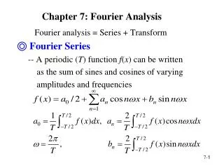
Chapter 7: Fourier Analysis. Fourier analysis = Series + Transform ◎ Fourier Series -- A periodic ( T ) function f ( x ) can be written as the sum of sines and cosines of varying amplitudes and frequencies. ○ Some function is formed by a finite number

E N D
Chapter 7: Fourier Analysis Fourier analysis = Series + Transform ◎ Fourier Series -- A periodic (T) function f(x) can be written as the sum of sines and cosines of varying amplitudes and frequencies
○ Some function is formed by a finite number of sinuous functions
Some function requires an infinite number of sinuous functions to compose
Spectrum The spectrum of a periodic function is discrete, consisting of components at dc, 1/T, and its multiples, e.g., For non-periodic functions, i.e., The spectrum of the function is continuous
○ In complex form: Compare with
Discrete case: ◎ Fourier Transform
Matrix form Let
Let ○ Inverse DFT
◎ Properties ○ Linearity: 。 Example: Noise removal f’ = f + n, n: noise, ○ Scaling
◎ Convolution: Convolution theorem:
◎ Correlation Correlation theorem
。Discrete Case: e.g., A = 4, B = 5, A + B – 1 = 8,
* Convolution can be defined in terms of polynomial product Extend f, g to if f, g have different numbers of sample points Let Compute The coefficients of to form the result of convolution
。Example: Let The coefficients of form the convolution
○ Fast Fourier Transform (FFT) -- Successive doubling method
。 Time complexity : the length of the input sequence FT: FFT: Times of speed increasing: N FT FFT Ratio 4 16 8 2.0 8 84 24 2.67 16 256 64 4.0 32 1024 160 6.4 64 4096 384 10.67 128 16384 896 18.3 256 65536 2048 32.0 512 262144 4608 56.9 1024 1048576 10240 102.4
○ Inverse FFT ← Given ← compute i. Input into FFT. The output is ii. Taking the complex conjugate and multiplying by N , yields the f(x)
◎ 2D Fourier Transform ○ FT: IFT:
◎ Properties ○ Filtering: every F(u,v) is obtained by multiplying every f(x,y) by a fixed value and adding up the results. DFT can be considered as a linear filtering ○ DC coefficient:
F(u,v) = F*(-u,-v) ○ Conjugate Symmetry:
○ Rotation Polor coordinates:
○ Display: effect of log operation
◎ Filtering in Frequency Domain ○ Low pass filtering I FT m IFT
D = 5 D = 30 ○ High pass filtering
◎ Butterworth Filtering ○ Low pass filter ○ High pass filter
○ Low pass filter ○ High pass filter
◎ Homomorphic Filtering -- Deals with images with large variation of illumination, e.g., sunshine + shadows -- Both reduces intensity range and increases local contrast ○ Idea: I = LR, L: illumination, R: Reflectance logI = logL + logR
low frequency high frequency
Euler’s formula: 7-44
○ Fast Fourier Transform (FFT) -- Successive doubling method Let Assume Let N = 2M. 7-47
] = ] ∵ = 7-48
Let --------- (B) Consider 7-49