Fourier Series
Fourier Series. Dr. K.W. Chow Mechanical Engineering. Introduction. Conceptual question: While one can readily see that two vectors can be ‘perpendicular’ or ‘orthogonal’, how can we extend this concept to a sequence of functions?. Introduction.

Fourier Series
E N D
Presentation Transcript
Fourier Series Dr. K.W. Chow Mechanical Engineering
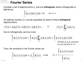
Introduction • Conceptual question: While one can readily see that two vectors can be ‘perpendicular’ or ‘orthogonal’, how can we extend this concept to a sequence of functions?
Introduction • A general formulation: For a sequence of functions {φn} and f(x) = Σcn φn What is cn? IF ∫ φm φn dx = 0 for m, n different, then cn can be found fromthis ‘orthogonal’ property.
Introduction • A general theory has been developed for linear, second order differential equations regarding these issues: (a) Orthogonal ‘eigenfunctions’? (b) Completeness in terms of expansion? (i.e. is it possible for any arbitrary function f(x) to be represented as a sum of φn(x)?)
Introduction • Sin(x) and Cos(x) are the solutions of the simplest second order ordinary differential equations (ODEs) • d2y/dx2 + y = 0, • subject to certain boundary conditions.
Introduction • Fourier series is an infinite series of sine and cosine • Dirichlet’s theorem (Sufficient, but not necessary): If a function is 2L-periodic and piecewise continuous, then its Fourier series converges • At a point of discontinuity, the series converges to the mean value.
Fourier series • an and bn are calculated by the orthogonal properties of sines and cosines. • If one uses a0 as the constant term, two schemes for defining an, n = 0and n > 0. • If one uses a0/2, then one definition for all an .
Introduction • Consider:
f(x) n = 3
f(x) n = 3 n = 7
f(x) n = 3 n = 7 n = 15
Introduction • The n = 15 series gives a very good approximation to the original function
Introduction Even function Odd function
Introduction • Even extension of a function results in Fourier cosine series • Odd extension of a function results in Fourier sine series (Assuming function is given only in half the interval.)
Introduction Even extension Odd extension
Introduction Even extension of f : Fourier series of f1will have cosine terms only Odd extension of f : Fourier series of f2will have sine terms only
Consider using odd extension
f(x) n = 3
f(x) n = 3 n = 7
f(x) n = 3 n = 7 n = 50
Introduction The Fourier series converges to this value at the discontinuity.
Introduction Approximation using n = 1 series
Introduction Approximation using n = 2 series
Introduction Approximation using n = 3 series
Introduction • Gibbs phenomenon – large oscillations of the series near a discontinuity.
Introduction • Consider the square wave again: 5 terms
Introduction 25 terms
Introduction 25 terms
Introduction • Animation to show the Gibbs phenomenon using different partial sums.
Differentiation of series • Fourier coefficients are determined uniquely using orthogonality of trigonometric functions. only when the series on the right is uniformly convergent. (d/dx = a local operator)
Integration of series • Always permitted, but the resulting series is not a Fourier series, unless the constant term a0 is zero. • (Integration = a global operator).
1D heat conduction in finite domain • Configuration: Density of conductor: Specific heat capacity: c Heat conduction coefficient: k Cross-sectional area: A Temperature: Temperature: L
1D heat conduction in finite domain Thermal conductivity defined by • Heat flux = - k A∂u/∂x where A = cross sectional area, u = temperature (i.e. k is heat flux per unit area per unit temperature gradient).
1D heat conduction in finite domain Assumptions: • Heat flow in the xdirection only • No external heat source • No heat loss
1D heat conduction in finite domain • Consider heat conduction across an infinitesimal element of the conductor: Heat out Heat in
1D heat conduction in finite domain • Heat flux at the left surface : - k A∂u(x,t)/∂x • Heat flux at the right surface: - k A ∂u(x,t)/∂x - ∂[k A ∂u(x,t)/∂x]/∂x dx + … • Net heat flux INTO the element: • ∂[k A ∂u(x,t)/∂x]/∂x dx
1D heat conduction in finite domain • Net heat must be used to heat up the element (c = specific heat capacity):
1D heat conduction in finite domain • Therefore (if k and A not functions of x):
1D heat conduction in finite domain • When , the above equation becomes exact: This is the 1D heat conduction equation in finite domain.
1D heat conduction in finite domain Solution procedure • Separation of variables: • Substitute back into the heat equation:
1D heat conduction in finite domain • Assume both ends are kept at : • For non-trivial solution, choose:
1D heat conduction in finite domain • F satisfies the differential equation: • For non-trivial solutions: • The temporal part:
1D heat conduction in finite domain • Overall solution: • Using superposition principle, we obtain general solution:
1D heat conduction in finite domain • is the Fourier sine coefficient:
1D heat conduction in finite domain • is called the eigen-value • is called the corresponding eigen-function
1D heat conduction in finite domain • Consider: