Genome-wide Study of Coordinative Gene Expression in Biological Processes
200 likes | 295 Vues
Explore how gene expression in interconnected biological processes is coordinated at the transcription level, using network analysis and correlation functions. Results showcase organized networks affecting cell cycle and stress response in yeast. Study methodology involves selecting processes, computing correlations, and identifying gene-level linkages. Gene Ontology terms and K–L divergence metrics are used to measure expressional association between processes. A randomization test assesses the significance of process associations.

Genome-wide Study of Coordinative Gene Expression in Biological Processes
E N D
Presentation Transcript
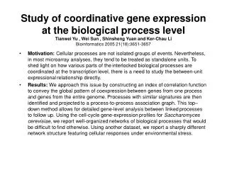
Study of coordinative gene expression at the biological process levelTianwei Yu , Wei Sun , Shinsheng Yuan and Ker-Chau LiBioinformatics 2005 21(18):3651-3657 • Motivation: Cellular processes are not isolated groups of events.Nevertheless, in most microarray analyses, they tend to be treatedas standalone units. To shed light on how various parts of theinterlocked biological processes are coordinated at the transcriptionlevel, there is a need to study the between-unit expressionalrelationship directly. • Results: We approach this issue by constructing an index ofcorrelation function to convey the global pattern of coexpressionbetween genes from one process and genes from the entire genome.Processes with similar signatures are then identified and projectedto a process-to-process association graph. This top–downmethod allows for detailed gene-level analysis between linkedprocesses to follow up. Using the cell-cycle gene-expressionprofiles for Saccharomyces cerevisiae, we report well-organizednetworks of biological processes that would be difficult tofind otherwise. Using another dataset, we report a sharply differentnetwork structure featuring cellular responses under environmentalstress.
Strategy of the study • Arrow a: select biological processes from the gene ontology system using a scheme described in Supplementary Figure 7. • Arrow b: compute correlations from large scale microarray data. • Arrow c: find gene level linkages between processes (this step may be skipped). • Arrow d: GIOC functions are established for each process. • Arrow e: use similarity between GIOC functions to measure the degree of expressional association between processes. • Arrow f: determine the significance of process association by randomization test. • Arrow g: connect associated processes and project the results as a graph.
Genome-wide index of correlation • For each GO term H, we create a probability function to serveas its GIOC. • Denote the collection of all yeast genes presentin the gene-expression dataset as G. • For each gene profile xiin G, we first evaluate its correlation with every gene profileyj in H. • The highest correlation, ci = maxjcorr(xi,yj), wherethe maximum is taken over all genes in H, indicates the levelof interaction between gene i and term H. • Using the clusteringanalysis terminology, this corresponds to the single linkagedistance measure between xi and all genes in term H. • We thenconvert ci into an index of correlation by a power functiontransformation. • Assign each gene i inG a probability mass pi (1+ci)6. Here the proportionality canbe determined by setting the total probability mass equal to1. • The resulting probability function PH(xi) = pi, i = 1,...,n,is called the GIOC function for term H.
GO term expressional association measure • The degree of expressional association between two GO termsH1 and H2 is determined by how similar their GIOC functionsare. We use K–L divergence between probability measuresto quantify the distance:
Randomization test of significance • We first specify the null hypothesis. • Suppose there are n genesin term H1, and m genes in term H2. To incorporate the casethat there may be genes that are annotated to both terms, wefurther assume that there are r overlap genes. • Under the nullhypothesis of no association between two terms, the m + n –r gene-expression profiles for these two terms should behaveas if they were randomly drawn from the entire gene-expressiondatabase. • To find the null distribution of the K–L distance,we use the Monte Carlo method. • Draw n+m–r profilesrandomly from the collection of all gene profiles. We use thefirst n of them to form one term and the last m of them to formthe second term. This naturally leads to r overlaps betweenthe two terms. • Compute the K–L distance betweenthese two artificially created terms. • This procedure is iteratedmany times to yield an approximation of the distribution ofK–L distance. • Once the null distribution is available,we can call a pair of GO terms significantly associated if theirK–L distance is shorter than a cutoff percentile.
Selecting GO terms to represent biological processes • Use the ‘biological process’ ontology for Saccharomycescerevisiae. • The GO system forms a directed acyclic graph. • Construct a representative set ofGO terms that do not have ancestor–descendent relationships. • This is because the analysis of a full size GO, which containsboth ancestor–descendent and sibling relationships, involvestoo much complexity and redundancy to yield easily interpretableresults. • Use computersearch to gain objectiveness. • Our program traverses the entire‘biological process’ branch of GO from top to bottom(Supplementary Figure 5). • A couple of parameters are optimizedto reach the dual aim of choosing terms as close to the bottomlevel as possible, and covering as many genes as possible. • Theresult is a collection C of 214 parallel terms. • This representativelist is at a scale finer than ‘GO slims’ (Ashburner et al., 2000;Dwight et al., 2002). The distribution of thenumber of genes in the selected terms is shown in SupplementaryFigure 6.
Within-GO term and between-GO term correlation structures • In order to find a proper measure of the expression associationbetween two GO terms, we first study how gene-expression profileswithin a GO term are correlated. We created an on-line GO termcomputation page (a module in http://kiefer.stat.ucla.edu/lap2)to facilitate the investigation. • Given a pair of terms X andY, the system computes gene-level correlations within each termand between the two terms. Subject to a user-specified sizelimit, the system also searches the entire genome for two listsof highest co-expressed genes, one for each term. • These twolists are then linked to the GO Term Finder of SGD to identifyenriched functional groups.
Not all genes from the sameGO term are tightly coexpressed. • To the contrary, the correlationswithin the majority of the terms we investigate are low (SupplementaryFigure 7); • e.g. the range is between –0.50 and 0.47 for‘actin cortical patch assembly’ (14 genes), • between–0.59 and 0.80 (median 0.03) for ‘axial budding’(21 genes), • and between –0.18 and 0.43 (median 0.19) for‘NAD biosynthesis’ (6 genes). • The correlations aremuch higher for terms involving translation mechanism, e.g.from –0.16 to 0.85 (median 0.53) for ‘ribosomallarge subunit biogenesis’ (14 genes).
yeast uses multipleintracellular or extracellular cues in regulating the resourcesdevoted to a functional module. • Despite the low average correlationwithin a GO term, each term has many strongly correlated genesfrom elsewhere of the genome; • but these genes are not highlycorrelated within themselves, and their cellular roles are diverse. • For instance, when we submit the top 200 genes which have thebest correlations (all >0.57) with ‘NAD biosynthesis’to GO Term Finder, no more than one-quarter of them fall intofunctionally enriched groups, the most visible ones being ‘catabolism’(27 genes), ‘protein folding’ (10 genes) and ‘regulationof protein metabolism’ (5 genes).
These preliminary findings argue for the merit of consideringGIOC function. • Our aim is to find a higher order organizationamong a diverse list of biological processes. • Therefore, inquantifying the degree of expressional association between apair of GO terms, we should not isolate the genes in the termpair from the rest of the genome. • The informationfrom genes outside of the two GO terms must be integrated first.
Expressional association in cell cycle data ComponentD shows an extensively connected network of metabolic processesincluding four major categories: coenzyme metabolism, aminoacid/lipid metabolism, small molecule transport/homeostasisand polysaccharide metabolism/energy generation. A :cell-cycle mechanism B:coherent operation within the translation mechanism C: features the proteintransport mechanism we find a totalof 202 GO-term associations significant at level 0.025.
Environmental stress gene expression data. Less connections are found. Section A features yeast's characteristic responses under stress. Section B features a cluster of ribosome/protein synthesis terms, together with a group of closely related metabolic terms.
GO-graph distance and expressional association. Boxplots showing the relationship between GO-graph distances and K–L distances. Proportion of expressionally associated pairs versus GO-graph distance. The GO-graph distance between two terms is the length of the shortest path between them, considering all edges as bi-directional. The K–L distances were computed from cell-cycle data.
Further discussion • We find two possible scenarios for a pair of terms to be linkedby our expressional measure: • (1) by tight coexpression betweentheir genes directly; • (2) by their shared co-expressed geneselsewhere in the genome. • Ribosome and translation related genesare known to be under tight cellular control. As expected, boththe within-term and the between-term correlations in componentB of Figure 2 are high.
In contrast, we find both the within-termand the between-term correlations in component D are much lower(Supplementary Figure 12). This indicates that multiple intracellularcues have been utilized to ensure the proper flow of metabolitesacross a variety of metabolic processes.
An example of the first scenario • In Supplementary Figure13a, the expression profiles for genes in the pair ‘rRNAmodification’ and ‘ribosomal large subunit biogenesis’(both 14 genes; no overlap) are compared by hierarchical clustering.Many cross-term neighbors are observed.
an example of the second scenario • Revisit the term ‘NADbiosynthesis’ in component D of Figure 2. • As one of thekey coenzymes involved in multiple metabolic pathways, the levelof NAD and NAD/NADH ratio is crucial for maintaining well-regulatedmetabolism. • Reflecting this important physiological relationship,our method finds a direct link between ‘NAD biosynthesis’and ‘NADH metabolism’ (6 and 7 genes respectively;no overlap). • In order to identify the source of the link, wefind the coexpressed genes for each term. • There are 463 genesthat have correlations of >0.5 with ‘NAD biosynthesis’,and 363 genes with ‘NADH metabolism’. The two groupsshare 117 genes. • These 117 genes serve as the bridges that linkthe two terms. However, there are only two cross-term correlations>0.5. • We note that the two terms share an ancestor ‘nicotinamidemetabolism’. Among the 13 genes that are annotated tothis ancestor but not to the two NAD terms, 11 are in the descendentterm ‘NADPH regeneration’ (no overlap with the twoNAD terms). However, ‘NADPH regeneration’ is connectedto neither of the two terms, and none of its 11 genes serveas a bridge for the two terms.
Another example • The pair ‘NAD biosynthesis’ and‘tricarboxylic acid cycle’ (6 and 14 genes respectively;no overlap). • It is well-known that multiple steps in the TCAcycle require NAD (Alberts et al., 2002) • Our method doesfind the link between these two terms. • There are 463 genes thathave correlations of >0.5 with ‘NAD biosynthesis’,and 566 genes with ‘tricarboxylic acid cycle’. • Thetwo groups share 207 genes. • However, there is only one cross-termcorrelation >0.5. • Supplementary Figure 13b and c show howthe clustering patterns in these two examples are differentfrom what is seen in Supplementary Figure 13a.