
Frequency Counts over Data Streams
E N D
Presentation Transcript
Frequency Countsover Data Streams Gurmeet Singh Manku Stanford University, USA VLDB 2002
The Problem ... Stream • Identify all elements whose current frequency exceeds support threshold s = 0.1%.
Stream • Identify all subsets of items whose current frequency exceeds s = 0.1%. Frequent Itemsets / Association Rules A Related Problem ...
Applications • Flow Identification at IP Router [EV01] • Iceberg Queries [FSGM+98] • Iceberg Datacubes [BR99 HPDW01] • Association Rules & Frequent Itemsets • [AS94 SON95 Toi96 • Hid99 HPY00 …]
3. Algorithm for Frequent Itemsets Presentation Outline ... 1. Lossy Counting 2. Sticky Sampling
Window 1 Window 2 Window 3 Algorithm 1: Lossy Counting Step 1: Divide the stream into ‘windows’ Is window size a function of support s? Will fix later…
Frequency Counts + First Window At window boundary, decrement all counters by 1 Lossy Counting in Action ... Empty
Frequency Counts + Next Window At window boundary, decrement all counters by 1 Lossy Counting continued ...
Error Analysis How much do we undercount? If current size of stream = N andwindow-size = 1/ε then #windows = εN frequency error Rule of thumb: Set ε = 10% of support s Example: Given support frequency s = 1%, set error frequency ε = 0.1%
Output: Elements with counter values exceeding sN – εN Approximation guarantees Frequencies underestimated by at most εN No false negatives False positives have true frequency at least sN – εN How many counters do we need? Worst case: 1/ε log (ε N) counters [See paper for proof]
Enhancements ... Frequency Errors For counter (X, c), true frequency in [c, c+εN] Trick: Remember window-id’s For counter (X, c, w), true frequency in [c, c+w-1] If (w = 1), no error! Batch Processing Decrements after k windows
Stream 28 31 41 34 15 30 23 35 19 Algorithm 2: Sticky Sampling Create counters by sampling Maintain exact counts thereafter What rate should we sample?
Approximation guarantees (probabilistic) Frequencies underestimated by at most εN No false negatives False positives have true frequency at least sN – εN Same error guarantees as Lossy Counting but probabilistic Sticky Sampling contd... For finite stream of length N Sampling rate = 2/Nε log 1/(s) = probability of failure Output: Elements with counter values exceeding sN – εN Same Rule of thumb: Set ε = 10% of support s Example: Given support threshold s = 1%, set error threshold ε = 0.1% set failure probability = 0.01%
Independent of N! Sampling rate? Finite stream of length N Sampling rate: 2/Nε log 1/(s) Infinite stream with unknown N Gradually adjust sampling rate (see paper for details) In either case, Expected number of counters = 2/ log 1/s
No of counters No of counters N (stream length) Sticky Sampling Expected: 2/ log 1/s Lossy Counting Worst Case: 1/ log N Support s = 1% Error ε = 0.1% Log10 of N (stream length)
From elements to setsof elements …
Stream Frequent Itemsets => Association Rules Frequent Itemsets Problem ... • Identify all subsets of items whose current frequency exceeds s = 0.1%.
Three Modules TRIE SUBSET-GEN BUFFER
45 50 40 31 29 32 42 30 50 40 30 31 29 45 32 42 Sets with frequency counts Module 1: TRIE Compact representation of frequent itemsets in lexicographic order.
In Main Memory Module 2: BUFFER Window 1 Window 2 Window 3 Window 4 Window 5 Window 6 Compact representation as sequence of ints Transactions sorted by item-id Bitmap for transaction boundaries
3 3 3 4 2 2 1 2 1 3 1 1 Frequency counts of subsets in lexicographic order Module 3: SUBSET-GEN BUFFER
3 3 3 4 2 2 1 2 1 3 1 1 SUBSET-GEN BUFFER TRIE new TRIE Overall Algorithm ... Problem: Number of subsets is exponential!
SUBSET-GEN Pruning Rules • A-priori Pruning Rule • If set S is infrequent, every superset of S is infrequent. • Lossy Counting Pruning Rule • At each ‘window boundary’ decrement TRIE counters by 1. • Actually, ‘Batch Deletion’: • At each ‘main memory buffer’ boundary, • decrement all TRIE counters by b. See paper for details ...
3 3 3 4 2 2 1 2 1 3 1 1 SUBSET-GEN BUFFER TRIE new TRIE Consumes main memory Consumes CPU time Bottlenecks ...
Design Decisions for Performance TRIE Main memory bottleneck Compact linear array (element, counter, level) in preorder traversal No pointers! Tries are on disk All of main memory devoted to BUFFER Pair of tries old and new (in chunks) mmap() and madvise() SUBSET-GEN CPU bottleneck Very fast implementation See paper for details
IBM synthetic dataset T10.I4.1000K N = 1Million Avg Tran Size = 10 Input Size = 49MB IBM synthetic dataset T15.I6.1000K N = 1Million Avg Tran Size = 15 Input Size = 69MB Frequent word pairs in 100K web documents N = 100K Avg Tran Size = 134 Input Size = 54MB Frequent word pairs in 806K Reuters newsreports N = 806K Avg Tran Size = 61 Input Size = 210MB Experiments ...
Three independent variables Fix one and vary two Measure time taken What do we study? For each dataset Support threshold s Length of stream N BUFFER size B Time taken t Set ε = 10% of support s
Varying support s and BUFFER B Time in seconds Time in seconds S = 0.004 S = 0.008 S = 0.001 S = 0.012 S = 0.002 S = 0.016 S = 0.004 S = 0.020 S = 0.008 BUFFER size in MB BUFFER size in MB IBM 1M transactions Reuters 806K docs Fixed: Stream length N Varying: BUFFER size B Support threshold s
Varying length N and support s S = 0.001 S = 0.002 S = 0.001 Time in seconds Time in seconds S = 0.004 S = 0.002 S = 0.004 Length of stream in Thousands Length of stream in Thousands IBM 1M transactions Reuters 806K docs Fixed: BUFFER size B Varying: Stream length N Support threshold s
Varying BUFFER B and support s Time in seconds Time in seconds B = 4 MB B = 4 MB B = 16 MB B = 16 MB B = 28 MB B = 28 MB B = 40 MB B = 40 MB Support threshold s Support threshold s IBM 1M transactions Reuters 806K docs Fixed: Stream length N Varying: BUFFER size B Support threshold s
Comparison with fast A-priori Dataset: IBM T10.I4.1000K with 1M transactions, average size 10. A-priori by Christian Borgelthttp://fuzzy.cs.uni-magdeburg.de/~borgelt/software.html
Comparison with Iceberg Queries Query: Identify all word pairs in 100K web documents which co-occur in at least 0.5% of the documents. [FSGM+98] multiple pass algorithm: 7000 seconds with 30 MB memory Our single-pass algorithm: 4500 seconds with 26 MB memory Our algorithm would be much faster if allowed multiple passes!
Lessons Learnt ... Optimizing for #passes is wrong! Small support s Too many frequent itemsets! Time to redefine the problem itself? Interesting combination of Theory and Systems.
Work in Progress ... • Frequency Counts over Sliding Windows • Multiple pass Algorithm for Frequent Itemsets • Iceberg Datacubes
Summary Lossy Counting: A Practical algorithm for online frequency counting. First ever single pass algorithm for Association Rules with user specified error guarantees. Basic algorithm applicable to several problems.
Thank you! http://www.cs.stanford.edu/~manku/research.html manku@stanford.edu
Sticky Sampling Expected: 2/ log 1/s Lossy Counting Worst Case: 1/ log N But ... LC: Lossy Counting SS:Sticky Sampling Zipf: Zipfian distribution Uniq: Unique elements