Competition and Market Equilibrium
940 likes | 1.26k Vues
Competition and Market Equilibrium. Perfect Competition. Defining Characteristic is lack of market power Price Takers How do we get there? Homogeneous output (or homogeneous enough)

Competition and Market Equilibrium
E N D
Presentation Transcript
Perfect Competition • Defining Characteristic is lack of market power • Price Takers • How do we get there? • Homogeneous output (or homogeneous enough) • Enough buyers and sellers that no one (or group thereof acting together) can effect demand or supply enough to affect market price • Perfect information (all participants know the market price) • Free entry and exit in the long run (to ensure price = MC)
Supply and Demand • The workhorse model of economics assumes perfectly competitive markets. • Seems odd since so few markets satisfy all conditions, but predictive power holds for markets that are less competitive.
Why do economists like them so much • With competitive markets, when all goods are private, there are no externalities and we don’t worry about income distribution… • Markets • Produce goods at the lowest possible cost (technical efficiency) • Commit all resources to their highest use (we produce the mix of goods people want as cheaply as possible) • Goods and services are consumed by those who value them most (maximize economic surplus, but not utility)
Technical Efficiency:Two Apple Growers of Many $ $ SMC $1.20 SMC $1.00 q* q* q q • Both farmers are producing at q* to start. Total cost of production can be lowered if Farmer Blue produces one fewer apple and Farmer Red produces one more. • To minimize total cost of producing apples, the SMC of the last apple produced by every farmer must be the same. • Perfectly competitive industries get this result.
Allocative EfficiencyRatio of market price = ratio of MC Oranges Qo Apples Qa
Wow! • Any and all units of a good or service that can be produced at an opportunity cost below the value of the good to consumers will be produced (and should be produced). • What coordinates all this magic? Price. • Price • signals opportunity cost of resources to producers so they can minimize cost and know how much to produce and when to enter or exit production. • Signals to consumers the value of the resources in production so that goods and services are consumed only by those whose value exceeds cost.
This IS the Invisible Hand • Adam Smith: • Efficient Resource Allocation: Markets minimize the cost of production (only the lowest cost producers produce) • Consumer Surplus Maximization: Markets maximize the consumer surplus in consumption (highest value consumers consume) • All and only units where benefit > cost will be produced • And not only in one market for one good, but for all markets and all goods* * except for those pesky market failures
Competition vs Non-competitive Markets • While prices create technical efficiency and promote efficient rationing in less than competitive situations, allocative efficiency is lacking (monopolists underproduce) • Only in perfect competition is economic surplus maximized. • MB=MC for last unit produced, no deadweight loss.
Demand • Demand is simply the horizontal sum of individual demand curves • No short vs long run… although… • Demand becomes more elastic over time as time allows individuals to find substitutes.
Market Demand • Assume a market with 3 individuals: x1 = 25 – 2px x2 = 45 – 1.5px x3 = 50 – 2.5px • The market demand curve is the horizontal sum X = 120 – 6px (P = 20-.143X) • Except for the kinks. This equation is for this line p 30 20 D 12.50 50 45 25 Q
Firm and Market Supply • Very Short Run: Quantities of all inputs are fixed. • Short Run: At least one input, but not all, are fixed. • Long Run: Quantities of all inputs used are variable.
Market Adjustment in the Very Short Run When quantity is fixed in the very short run and demand increases, price will rise but quantity will not change as firms cannot increase production. P VSRS SRS Demand for plywood increases as a hurricane approaches. D’ D Q
Market Adjustment in the Very Short Run P Similarly, there can be a supply shock (e.g. hurricane) that shifts supply back S’ S D Q
Market Adjustment in the Very Short Run P Gasoline: Price rises with supply shift. Assume an excise tax on gasoline. Politicians call for suspending the tax, but in the short run price will be unaffected as neither supply or demand would shift as a result. S’ S Tax Tax D Q
Market Adjustment in the Very Short Run P Gasoline: Price rises with supply shift. Assume an excise tax on gasoline. Politicians call for suspending the tax, but in the short run price will be unaffected as neither supply or demand would shift as a result. S’ S Tax D Q
Short Run/Long Run Model • The more usual analysis. • Short Run • Firms produce where MR = SMC • Firms may shut down in the short run • Market supply is the horizontal sum of all firms in the industry (no entry or exit in the short run) • Long Run • Price driven to the break-even price as firms enter/exit to seek profits and avoid losses • Profits = 0 • Firm on expansion path • Capital at the level that minimizes SAC
Long and Short Run Cost Curves • Assume we start here. MC $ SMC SAC AC AVC q
Short Run • Short Run supply is SMC at P > min(AVC) • Yes, firms will produce at lower prices in SR than LR. $ SMC MC SAC AC SAVC q
Short Run, Firm and Market • Assume we start here for short run. SMC $ $ SRS SAC SAVC PSD D q q
Long Run • Assume IRS and then DRS (no CRS) $ SMC MC SAC AC AVC q
Firm Long Run Supply • q where P = MC so long as π ≥0 (P> PBE) $ Firm LRS AC MC PBE q
Long Run Market Supply • Long run firm supply: q=4P • So long run market supply: Q=N(4P)? • NO!!!
Long Run Firms Enter and Exit until profit = 0 and market price = PBE • In long run: P →PBE and π →0 $ MC AC PBE q qLR
Long Run Market Supply Assumes constant cost industry, more to come on that! • Firms enter and exit so that in the long run, LRS = the quantity demanded at the pBE SMC P P S MC SAC AC PBE LRS PSD D q Q
Shocks • Change in demand • Change in FC • Change in VC
Change in Demand • Short Run: price up, Δ Q is n*Δq, π > 0 SMC SRS1 $ $ ATC AVC PBE D D q Q q1 q2 Q2 Q1
Change in Demand • Long run: Firms enter, π > 0 SMC SRS1 $ $ SRS2 ATC AVC PBE D D q Q q1 q2 Q2 Q3
Change in Demand • Long Run Supply: If the PBE does not change, the market will always supply the Qd at PBE . SMC $ $ SRS2 ATC AVC LRS PBE D D q Q q1 Q3
Comparative Statics Analysis • In the long run, the number of firms in the industry will vary from one long-run equilibrium to another • Assume that we are examining a constant-cost industry • Suppose that the initial long-run equilibrium industry output is Q0 and the typical firm’s output is q* (where AC is minimized) • The equilibrium number of firms in the industry N1 = Q1/q1*
Comparative Statics Analysis • A shift in demand that changes the equilibrium industry output to Q3 will change the equilibrium number of firms to N3 = Q3/q1* • The change in the number of firms is • In a constant cost industry q*will not change, so only the size of the shift in demand will affect the change in n.
Change in FC • Short Run: MC is unaffected, so qs is unaffected, so PM is unaffected. But firms suffer losses. SMC SRS1 $ $ ATC AVC PBE D q Q q1 Q1
Change in FC • Long run: Firms exit until the PM = the new PBE . • With higher price of K, firms use less. • Change in firm level of output is unknown. ATC’ SMC’ SRS1 $ $ AVC’ PBE2 PBE1 D q Q q3 Q1
Change in FC • Long run: Firms exit until the PM = the new PBE. SMC’ SRS1 $ $ SAC’ AVC’ LRS2 PBE2 LRS1 PBE1 D q Q q3 Q1 Q3
Change in VC • Short Run: MC is affected, so qs is affected, as is PM . Firms suffer losses, as the higher price does not cover the higher cost. SMC SRS1 $ $ ATC AVC PBE D q Q q1 Q1 If AVC > P, firms will shut down.
Change in VC • While firm supply decreases, qs is unknown as we don’t know the change in price. However, change in MC > change in P. SRS2 SMC SRS1 $ $ ATC AVC PBE D q Q q1 Q1 Q2 If AVC > P, firms will shut down.
Change in VC • Again, with higher costs, and PBE, the LRS curve will shift upwards. The new q* (and optimal K) could be higher or lower. SRS3 SRS2 SMC SRS1 $ $ ATC AVC LRS2 PBE2 LRS1 PBE1 D q Q q3 Q1 Q3
Comparative Statics Analysis • The effect of a change in input prices • we need to know how much minimum average cost is affected • we need to know how an increase in long-run equilibrium price will affect quantity demanded
Comparative Statics Analysis • The optimal level of output for each firm may also be affected • Therefore, the change in the number of firms becomes • And the relative changes in Q and q* will determine the change in N.
Supply and Demand • Basis is the competitive model • Usually, competitive market in the short run. • Sometimes used to depict competitive market in the long run with increasing cost industry assumption. • Treatment • Algebra (to get equilibrium) • Calculus (comparative statics) • Demand shifters • Supply shifters • Sales and Excise taxes
As in Intermediate Micro • Inverse Demand: P = 1,500 - .5Qd • Inverse Supply: P = 600 + Qs • Solution is Q = 600, P = 1,200 P S 1,500 1,200 D 600 Q 600 3,000
Sales Tax, Comparative Statics • Intermediate • Add Sales Tax = $150 • Inverse Demand: P = 1500 - tax - .5Qd • Inverse Supply: P = 600 + Qs • Solution is Q = 500, P = 1100 (consumer cost = P + t = $1250) • Just by comparing outcomes, P S Market Price PD=1,250 P*=1,100 D Dt Q 500
Excise Tax, Comparative Statics Market Price • Intermediate • Add Excise Tax = $150 • Inverse Demand: P = 1500 - .5Qd • Inverse Supply: P = 600 + tax + Qs • Solution is Q = 500, P = 1250 (producer keeps = P – t = $1100) • Just by comparing outcomes, P St S P*=1,250 PS=1,100 D Q 500
Linear Supply and Demand, Equilibrium • General linear functions specified • Inverse Demand: P = a – bQd (a > 0, b > 0) • Inverse Supply: P = c + dQs (c > 0, d > 0) • Equilibrium condition: Qs = Qd (and Ps = Pd) • Reduced form solution (only in terms of a, b, c, d) P a slope = d S P* slope = -b D c Q* Q
Shifts in Supply or Demand, Comparative Statics P a slope = d • Solution • Comparative Statics S P* slope = -b D c Q* Q Note, “b” rising means demand must be getting steeper. So long as a>c
Sales Tax • Market Model (sales tax) • Inverse Demand: P = a - t – bQd(a > 0, b > 0) • Inverse Supply: P = c + dQs (c > 0, d > 0) • Equilibrium condition: Qs = Qd • Reduced form solution (only in terms of a, b, c, d, t) P a S a-t PD* P* Pt* D c Dt Qt* Q* Q
