Approaching multiple sequence alignment from a phylogenetic perspective
580 likes | 597 Vues
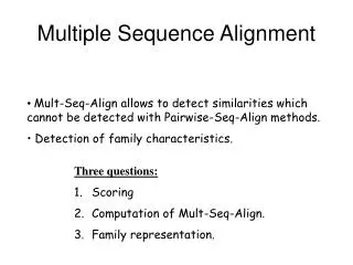
Explore approaches to multiple sequence alignment from a phylogenetic viewpoint. Learn about species phylogeny, life evolution, and Biomedical applications. Discover the latest algorithms, software, mathematics, and tools for large-scale phylogenetic research.

Approaching multiple sequence alignment from a phylogenetic perspective
E N D
Presentation Transcript
Approaching multiple sequence alignment from a phylogenetic perspective Tandy Warnow Department of Computer Sciences The University of Texas at Austin
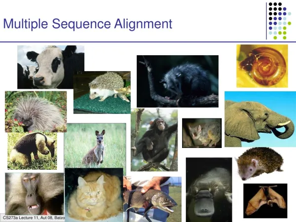
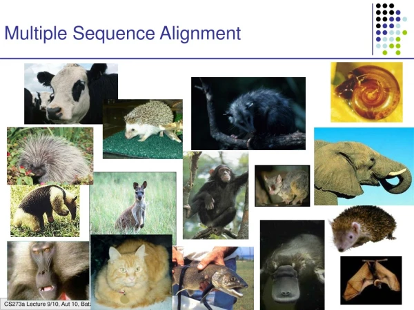
Species phylogeny From the Tree of the Life Website,University of Arizona Orangutan Human Gorilla Chimpanzee
How did life evolve on earth? An international effort to understand how life evolved on earth Biomedical applications: drug design, protein structure and function prediction, biodiversity Phylogenetic estimation is a “Grand Challenge”: millions of taxa, NP-hard optimization problems • Courtesy of the Tree of Life project
The CIPRES Project (Cyber-Infrastructure for Phylogenetic Research)www.phylo.org This project is funded by the NSF under a Large ITR grant • ALGORITHMS and SOFTWARE: scaling to millions of sequences (open source, freely distributed) • MATHEMATICS/PROBABILITY/STATISTICS: Obtaining better mathematical theory under complex models of evolution • DATABASES: Producing new database technology for structured data, to enable scientific discoveries • SIMULATIONS: The first million taxon simulation under realistically complex models • OUTREACH: Museum partners, K-12, general scientific public • PORTAL available to all researchers
Step 1: Gather data S1 = AGGCTATCACCTGACCTCCA S2 = TAGCTATCACGACCGC S3 = TAGCTGACCGC S4 = TCACGACCGACA
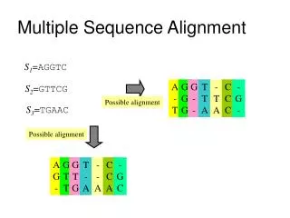
Step 2: Multiple Sequence Alignment S1 = AGGCTATCACCTGACCTCCA S2 = TAGCTATCACGACCGC S3 = TAGCTGACCGC S4 = TCACGACCGACA S1 = -AGGCTATCACCTGACCTCCA S2 = TAG-CTATCAC--GACCGC-- S3 = TAG-CT-------GACCGC-- S4 = -------TCAC--GACCGACA
Step 3: Construct tree S1 = AGGCTATCACCTGACCTCCA S2 = TAGCTATCACGACCGC S3 = TAGCTGACCGC S4 = TCACGACCGACA S1 = -AGGCTATCACCTGACCTCCA S2 = TAG-CTATCAC--GACCGC-- S3 = TAG-CT-------GACCGC-- S4 = -------TCAC--GACCGACA S1 S2 S4 S3
But molecular phylogenetics assumes the alignment is given S1 = -AGGCTATCACCTGACCTCCA S2 = TAG-CTATCAC--GACCGC-- S3 = TAG-CT-------GACCGC-- S4 = -------TCAC--GACCGACA S1 S2 S4 S3
This talk • DCM-NJ: Dramatic improvement in phylogeny estimation in terms of tree accuracy, and theoretical performance under Markov models of evolution • DCM-MP and DCM-ML: Speeding up heuristics for large-scale phylogenetic estimation • Simulation studies of two-phase methods (amino-acid and DNA sequences). • SATe: A new technique for simultaneous estimation of trees and alignments
Performance criteria • Estimated alignments are evaluated with respect to the true alignment. Studied both in simulation and on real data. • Estimated trees are evaluated for “topological accuracy” with respect to the true tree. Typically studied in simulation. • Methods for these problems can also be evaluated with respect to an optimization criterion (e.g., maximum likelihood score) as a function of running time. Typically studied on real data. (Reasonably valid for phylogeny but not yet for alignment.) Issues: Simulation studies need to be based upon realistic models, and “truth” is often not known for real data.
-3 mil yrs AAGACTT AAGACTT -2 mil yrs AAGGCCT AAGGCCT AAGGCCT AAGGCCT TGGACTT TGGACTT TGGACTT TGGACTT -1 mil yrs AGGGCAT AGGGCAT AGGGCAT TAGCCCT TAGCCCT TAGCCCT AGCACTT AGCACTT AGCACTT today AGGGCAT TAGCCCA TAGACTT AGCACAA AGCGCTT AGGGCAT TAGCCCA TAGACTT AGCACAA AGCGCTT DNA Sequence Evolution
Markov models of single site evolution Simplest (Jukes-Cantor): • The model tree is a pair (T,{e,p(e)}), where T is a rooted binary tree, and p(e) is the probability of a substitution on the edge e. • The state at the root is random. • If a site changes on an edge, it changes with equal probability to each of the remaining states. • The evolutionary process is Markovian. More complex models (such as the General Markov model) are also considered, often with little change to the theory.
FN FN: false negative (missing edge) FP: false positive (incorrect edge) 50% error rate FP
Statistical consistency, exponential convergence, and absolute fast convergence (afc)
Neighbor joining (although statistically consistent) has poor performance on large diameter trees [Nakhleh et al. ISMB 2001] Simulation study based upon fixed edge lengths, K2P model of evolution, sequence lengths fixed to 1000 nucleotides. Error rates reflect proportion of incorrect edges in inferred trees. 0.8 NJ 0.6 Error Rate 0.4 0.2 0 0 400 800 1200 1600 No. Taxa
Optimal labeling on a fixed tree can be computed in linear time O(nk) GTA ACA ACA GTA 2 1 1 ACT GTT MP score = 4 MP is not statistically consistent. Finding the optimal MP tree is NP-hard. Maximum Parsimony:
Maximum Likelihood (ML) • Given: stochastic model of sequence evolution (e.g. Jukes-Cantor) and a set S of sequences • Objective: Find tree T and parameter values so as to maximize the probability of the data. NP-hard, but statistically consistent. Preferred by many systematists, but even harder than MP in practice. (Exponential sequence lengths suffice for accuracy with high probability.)
Local optimum Cost Global optimum Phylogenetic trees Approaches for “solving” MP (and other NP-hard problems in phylogeny) • Hill-climbing heuristics (which can get stuck in local optima) • Randomized algorithms for getting out of local optima • Approximation algorithms for MP (based upon Steiner Tree approximation algorithms).
Problems with current techniques for MP and ML Shown here is the performance of a very good heuristic (TNT) for maximum parsimony analysis on a real dataset of almost 14,000 sequences. (“Optimal” here means best score to date, using any method for any amount of time.) Acceptable error is below 0.01%. Performance of TNT with time
Problems with existing phylogeny reconstruction methods • Polynomial time methods (generally based upon distances) have poor accuracy with large diameter datasets. • Heuristics for NP-hard optimization problems take too long (months to reach acceptable local optima).
Warnow et al.: Meta-algorithms for phylogenetics • Basic technique: determine the conditions under which a phylogeny reconstruction method does well (or poorly), and design a divide-and-conquer strategy to improve the performance • The divide-and-conquer technique is specific to the method. • Warnow et al. developed a class of divide-and-conquer methods, collectively called DCMs (Disk-Covering Methods).
Improving phylogeny reconstruction methods using DCMs • Improving the theoretical convergence rate and performance of polynomial time distance-based methods using DCM1 • Speeding up heuristics for NP-hard optimization problems (Maximum Parsimony and Maximum Likelihood) using Rec-I-DCM3
Neighbor joining (although statistically consistent) has poor performance on large diameter trees [Nakhleh et al. ISMB 2001] Simulation study based upon fixed edge lengths, K2P model of evolution, sequence lengths fixed to 1000 nucleotides. Error rates reflect proportion of incorrect edges in inferred trees. 0.8 NJ 0.6 Error Rate 0.4 0.2 0 0 400 800 1200 1600 No. Taxa
DCM1-boosting distance-based methods[Nakhleh et al. ISMB 2001] • Theorem: DCM1-NJ converges to the true tree from polynomial length sequences 0.8 NJ DCM1-NJ 0.6 Error Rate 0.4 0.2 0 0 400 800 1200 1600 No. Taxa
Problems with current techniques for MP Shown here is the performance of a TNT heuristic maximum parsimony analysis on a real dataset of almost 14,000 sequences. (“Optimal” here means best score to date, using any method for any amount of time.) Acceptable error is below 0.01%. Performance of TNT with time
Rec-I-DCM3 significantly improves performance (Roshan et al.) Current best techniques DCM boosted version of best techniques Comparison of TNT to Rec-I-DCM3(TNT) on one large dataset
Very nice, but… • Evolution is not as simple as these models assert!
indels (insertions and deletions) also occur! Deletion Mutation …ACGGTGCAGTTACCA… …ACCAGTCACCA…
Basic Questions • Does improving the alignment lead to an improved phylogeny? • Are we getting good enough alignments from MSA methods? • Are we getting good enough trees from the phylogeny reconstruction methods? • Can we improve these estimations, perhaps through simultaneous estimation of trees and alignments?
Multiple Sequence Alignment AGGCTATCACCTGACCTCCA TAGCTATCACGACCGC TAGCTGACCGC -AGGCTATCACCTGACCTCCA TAG-CTATCAC--GACCGC-- TAG-CT-------GACCGC-- Notes: 1. We insert gaps (dashes) to each sequence to make them “line up”. 2. Nucleotides in the same column are presumed to have a common ancestor (i.e., they are “homologous”).
Indels and substitutions at the DNA level Deletion Mutation …ACGGTGCAGTTACCA…
Indels and substitutions at the DNA level Deletion Mutation …ACGGTGCAGTTACCA…
Indels and substitutions at the DNA level Deletion Mutation …ACGGTGCAGTTACCA… …ACCAGTCACCA…
Deletion Mutation The true pairwise alignment is: …ACGGTGCAGTTACCA… …AC----CAGTCACCA… …ACGGTGCAGTTACCA… …ACCAGTCACCA… The true multiple alignment on a set of homologous sequences is obtained by tracing their evolutionary history, and extending the pairwise alignments on the edges to a multiple alignment on the leaf sequences.
Basics about alignments • The standard alignment method for phylogeny is Clustal (or one of its derivatives), but many new alignment methods have been developed by the protein alignment community. • Alignments are generally evaluated in comparison to the “true alignment”, using the SP-score (percentage of truly homologous pairs that show up in the estimated alignment). • On the basis of SP-scores (and some other criteria), methods like ProbCons, Mafft, and Muscle are generally considered “better” than Clustal.
Questions • Many new MSA methods improve on ClustalW on biological benchmarks (e.g., BaliBASE) and in simulation. Does this lead to improved phylogenetic estimations? • The phylogeny community has tended to assume that alignment has a big impact on final phylogenetic accuracy. But does it? Does this depend upon the model conditions? • What are the best two-phase methods?
Our simulation studies (both using ROSE*) • Amino-acid evolution (Wang et al., unpublished): Model trees based upon BaliBase and random birth-death trees, with 12 taxa to 100 taxa. Average gap length 3.4. Average identity ranges from 23% to 57%. Average gappiness ranges from 3% to 60%. • DNA sequence evolution (Liu et al., unpublished): Random birth-death trees, 25 to 500 taxa. Two gap length distributions (short and long). Average p-distance ranges from 43% to 63%. Average gappiness ranges from 40% to 80%. *ROSE has limitations!
Non-coding DNA evolution Models 1-4 have “long gaps”, and models 5-8 have “short gaps”
Observations • Phylogenetic tree accuracy is positively correlated with alignment accuracy (measured using SP), but the degree of improvement in tree accuracy is much smaller. (However, note that sometimes “worse” alignments yield better trees.) • The best two-phase methods are generally (but not always!) obtained by using either ProbCons or MAFFT, followed by ML. • However, even the best two-phase methods don’t do well enough.
Two problems with two-phase methods • All current methods for multiple alignment have high error rates when sequences evolve with many indels and substitutions. • All current methods for phylogeny estimation treat indel events inadequately (either treating as missing data, or giving too much weight to each gap).
Simultaneous estimation? • Statistical methods (e.g., AliFritz and BaliPhy) cannot be applied to datasets above ~20 sequences. • POY (Wheeler et al.) attempts to find tree/alignment pairs of minimum total edit distance. POY can be applied to larger datasets, but has not performed as well as the best two-phase methods.
SATe: (Simultaneous Alignment and Tree Estimation) • Developers: Warnow, Linder, Liu, Nelesen, and Zhao. • Search strategy: search through tree space, and align sequences on each tree by heuristically estimating ancestral sequences. • SATe-TL is the alignment/tree pair of minimum total length (default affine gap penalty has gap-open cost 2, gap-extend cost 0.5 and mismatch cost 1). • SATe-ML is the alignment/tree pair that optimizes maximum likelihoodunder GTR+Gamma+I.
Simulation study • 100 taxon model trees (generated by r8s and then modified, so as to deviate from the molecular clock). • DNA sequences evolved under ROSE (indel events of blocks of nucleotides, plus HKY site evolution). The root sequence has 1000 sites. • We vary the gap length distribution, probability of gaps, and probability of substitutions, to produce 8 model conditions: models 1-4 have “long gaps” and 5-8 have “short gaps”.
SATe-TL vs. SATe-ML vs. Clustal • Model conditions 1-4 have long gaps (100 taxa) • Model conditions 5-8 have short gaps (100 taxa)
Comments • The affine gap penalty matters! (Performance of SATe-TL for simple gap penalties is not as good.) • SATe-ML produces trees that are more accurate than SATe-TL, and both improve upon trees estimated using Clustal (contrary to Ogden and Rosenberg’s 2007 Systematic Biology paper). What about comparisons to other two-phase methods?
Our method (SATe-ML) vs. other methods • Long gap models 1-4, Short gap models 5-8
Alignment accuracy FN: proportion of correctly homologous pairs of nucleotides missing from the estimated alignment (i.e., 1-SP score). FP: proportion of incorrect pairings of nucleotides in the estimated alignment.