Anna M. Michalak Department of Civil and Environmental Engineering

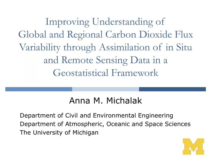
1. Improving Understanding of Global and Regional Carbon Dioxide Flux Variability through Assimilation of in Situ and Remote Sensing Data in a Geostatistical Framework Anna M. Michalak Department of Civil and Environmental Engineering Department of Atmospheric, Oceanic and Space Sciences The University of Michigan

2. Outline • Introduction to geostatistics • Inverse modeling approaches to estimating flux distributions • Geostatistical approach to quantifying fluxes: • Global flux estimation • Use of auxiliary data • Regional scale synthesis

3. Spatial Correlation • Measurements in close proximity to each other generally exhibit less variability than measurements taken farther apart. • Assuming independence, spatially-correlated data may lead to: • Biased estimates of model parameters • Biased statistical testing of model parameters • Spatial correlation can be accounted for by using geostatistical techniques

4. Parameter Bias Example map of an alpine basin Q: What is the mean snow depth in the watershed? snow depth measurements kriging estimate of mean snow depth (assumes spatial correlation) mean of snow depth measurements (assumes spatial independence)

5. 5% H0 Rejected H0 Rejected! H0 is TRUE 5% H0 Rejected H0Not Rejected 5% H0 rejected

6. Variogram Model • Used to describe spatial correlation 1 2 3 4

7. Geostatistics in Practice • Main uses: • Data integration • Numerical models for prediction • Numerical assessment (model) of uncertainty

8. Geostatistical Inverse Modeling Actual flux history Available data

9. Geostatistical Inverse Modeling Geostatistical Bayesian / Independent Errors 31 data 201 fluxes 31 data 101 fluxes 31 data 41 fluxes 31 data 11 fluxes 31 data 21 fluxes

10. Key Points • If the parameter(s) that you are modeling exhibits spatial (and/or temporal) autocorrelation, this feature must be taken into account to avoid biased solutions • Spatial (and/or temporal) autocorrelation can be used as a source of information in helping to constrain parameter distributions • The field of geostatistics provides a framework for addressing the above two issues

11. Factors such as clouds, aerosols and computational limitations limit sampling for existing and upcoming satellite missions such as the Orbiting Carbon Observatory A sampling strategy based on XCO2 spatial structure assures that the satellite gathers enough information to fill data gaps within required precision ASIDE: CO2 Measurements from Space Alkhaled et al. (in prep.)

12. x104 km XCO2 Variability • Regional spatial covariance structure is used to evaluate: • Regional sampling densities required for a set interpolation precision • Minimum sampling requirements and optimal sampling locations

13. Source: NOAA-ESRL

14. -24 hours -48 hours -72 hours -96 hours -120 hours What Surface Fluxes do Atmospheric Measurements See? 24 June 2000: Particle Trajectories Latitude Height Above Ground Level (km) Longitude Longitude Source: Arlyn Andrews, NOAA-GMD

15. Need for Additional Information • Current network of atmospheric sampling sites requires additional information to constrain fluxes: • Problem is ill-conditioned • Problem is under-determined (at least in some areas) • There are various sources of uncertainty: • Measurement error • Transport model error • Aggregation error • Representation error • One solution is to assimilate additional information through a Bayesian approach

16. Bayesian Inference Applied to Inverse Modeling for Surface Flux Estimation Likelihood of fluxes given atmospheric distribution Posterior probability of surface flux distribution Prior information about fluxes p(y) probabilityofmeasurements y : available observations (n×1) s: surface flux distribution (m×1)

17. Synthesis Bayesian Inversion Prior flux estimates (sp) BiosphericModel CO2Observations (y) AuxiliaryVariables Inversion Flux estimates and covarianceŝ, Vŝ ? TransportModel Sensitivity of observations to fluxes (H) Meteorological Fields Residual covariancestructure (Q, R) ?

18. Large Regions Inversion TransCom, Gurney et al. 2003

19. Transport Model Gridscale Inversions Rödenbeck et al. 2003

20. Variogram Model • Used to describe spatial correlation 1 2 3 4

21. Geostatistical Approach to Inverse Modeling • Geostatistical inverse modeling objective function: • H = transport information, s = unknown fluxes, y = CO2 measurements • X and  define the model of the trend • R = model data mismatch covariance • Q = spatio-temporal covariance matrix for the flux deviations from the trend Deterministic component Stochastic component

22. Synthesis Bayesian Inversion Prior flux estimates (sp) BiosphericModel CO2Observations (y) AuxiliaryVariables Inversion Flux estimates and covarianceŝ, Vŝ TransportModel Sensitivity of observations to fluxes (H) Meteorological Fields Residualcovariancestructure (Q, R)

23. Geostatistical Inversion select significant variables AuxiliaryVariables VarianceRatioTest CO2Observations (y) Flux estimates and covariance ŝ, Vŝ Inversion TransportModel Sensitivity of observations to fluxes (H) Trend estimate and covariance β, Vβ Meteorological Fields Residual covariancestructure (Q, R) RMLOptimization optimize covariance parameters

24. Key Questions • Can the geostatistical approach estimate: • Sources and sinks of CO2 without relying on prior estimates? • Spatial and temporal autocorrelation structure of residuals? • Significance of available auxiliary data? • Relationship between auxiliary data and flux distribution? • If so, what do we learn about: • Flux variability (spatial and temporal) • Influence of prior flux estimates in previous studies • Impact of aggregation error • What are the opportunities for further expanding this approach to move from attribution to diagnosis and prediction?

25. Fluxes Used in Pseudodata Study Michalak, Bruhwiler & Tans (JGR, 2004)

26. Recovery of Annually Averaged Fluxes Best estimate “Actual” fluxes Michalak, Bruhwiler & Tans (JGR, 2004)

27. Recovery of Annually Averaged Fluxes Best estimate Standard Deviation Michalak, Bruhwiler & Tans (JGR, 2004)

28. Key Questions • Can the geostatistical approach estimate • Sources and sinks of CO2 without relying on prior estimates? • Spatial and temporal autocorrelation structure of residuals? • Significance of available auxiliary data? • Relationship between auxiliary data and flux distribution? • If so, what do we learn about: • Flux variability (spatial and temporal) • Influence of prior flux estimates in previous studies • Impact of aggregation error • What are the opportunities for further expanding this approach to move from attribution to diagnosis and prediction?

29. Auxiliary Data and Carbon Flux Processes Other: Spatial trends (sine latitude, absolute value latitude) Environmental parameters: (precipitation, %landuse, Palmer drought index) Anthropogenic Flux: Fossil fuel combustion (GDP density, population) Oceanic Flux: Gas transfer (sea surface temperature, air temperature) Terrestrial Flux: Photosynthesis (FPAR, LAI, NDVI) Respiration (temperature) Image Source: NCAR

30. Sample Auxiliary Data Gourdji et al. (in prep.)

31. Which Model is Best?

32. Geostatistical Approach to Inverse Modeling • Geostatistical inverse modeling objective function: • H = transport information, s = unknown fluxes, y = CO2 measurements • X and  define the model of the trend • R = model data mismatch covariance • Q = spatio-temporal covariance matrix for the flux deviations from the trend Deterministic component Stochastic component

33. Global Gridscale CO2 Flux Estimation • Estimate monthly CO2 fluxes (ŝ) and their uncertainty on 3.75° x 5° global grid from 1997 to 2001 in a geostatistical inverse modeling framework using: • CO2 flask data from NOAA-ESRL network (y) • TM3 (atmospheric transport model) (H) • Auxiliary environmental variables correlated with CO2 flux • Three models of trend flux (Xβ) considered: • Simple monthly land and ocean constants • Terrestrial latitudinal flux gradient and ocean constants • Terrestrial gradient, ocean constants and auxiliary variables

34. Measurement Locations Gourdji et al. (in prep.) Mueller et al. (in prep.)

35. Selected Auxiliary Variables Combine physical understanding with results of VRT to choose final set of auxiliary variables: % Ag LAI SST % Forest fPAR dSSt/dt % Shrub NDVI Palmer Drought Index % Grass Precipitation GDP Density Land Air Temp. Population Density Combine physical understanding with results of VRT to choose final set of auxiliary variables: % AgLAISST % ForestfPARdSSt/dt % ShrubNDVI Palmer Drought Index % Grass PrecipitationGDP Density Land Air Temp.Population Density Inversion estimates drift coefficients (β): Gourdji et al. (in prep.)

36. Building up the best estimate in January 2000 Deterministic component Stochastic component Gourdji et al. (in prep.)

37. A posteriori uncertainty for January 2000 Gourdji et al. (in prep.)

38. Transcom Regions TransCom, Gurney et al. 2003

39. Regional comparison of seasonal cycle Gourdji et al. (in prep.)

40. Regional comparison of seasonal cycle #2 Gourdji et al. (in prep.)

41. Comparison of annual average non-fossil fuel flux Gourdji et al. (in prep.)

42. Key Questions • Can the geostatistical approach estimate • Sources and sinks of CO2 without relying on prior estimates? • Spatial and temporal autocorrelation structure of residuals? • Significance of available auxiliary data? • Relationship between auxiliary data and flux distribution? • If so, what do we learn about: • Flux variability (spatial and temporal) • Influence of prior flux estimates in previous studies • Impact of aggregation error • What are the opportunities for further expanding this approach to move from attribution to diagnosis and prediction?

43. Opportunities for Regional Synthesis Continuous tall-tower data available More consistent relationship to auxiliary variables Flux tower and aircraft campaign data available for validation NACP offers opportunities for intercomparison / collaborations Photo credit: B. Stephens, UND Citation crew, COBRA WLEF tall tower (447m) in Wisconsin with CO2 mixing ratio measurements at 11, 30, 76, 122, 244 and 396 m

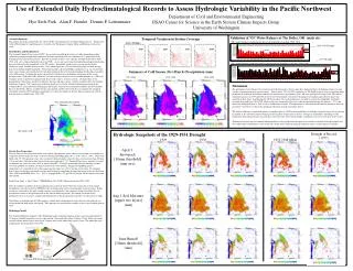
44. North American CO2 Flux Estimation • Estimate North American CO2 fluxes at 1°x1° resolution & daily/weekly/monthly timescales using: • CO2 concentrations from 3 tall towers in Wisconsin (Park Falls), Maine (Argyle) and Texas (Moody) • STILT – Lagrangian atmospheric transport model • Auxiliary remote-sensing and in situ environmental data Pseudodata and recovered fluxes (Source: Adam Hirsch, NOAA-ESRL)

45. Assimilation of Remote Sensing and Atmospheric Data Analysis steps: • Compile auxiliary variables • Select significant variables to include in model of the trend • Estimate covariance parameters: • Model-data mismatch • Flux deviations from overall trend. • Perform inversion, estimating both (i) the relationship between auxiliary variables and flux , and (ii) the flux distribution s. • A posteriori covariance includes the uncertainties of fluxes, trend parameters, and all cross-covariances

46. Key Questions • Can the geostatistical approach estimate • Sources and sinks of CO2 without relying on prior estimates? • Spatial and temporal autocorrelation structure of residuals? • Significance of available auxiliary data? • Relationship between auxiliary data and flux distribution? • If so, what do we learn about: • Flux variability (spatial and temporal) • Influence of prior flux estimates in previous studies • Impact of aggregation error • What are the opportunities for further expanding this approach to move from attribution to diagnosis and prediction?

47. Conclusions • Atmospheric data information content is sufficient to: • Quantify model-data mismatch and flux covariance structure • Identify significant auxiliary environmental variables and estimate their relationship with flux • Constrain continental fluxes independently of biospheric model and oceanic exchange estimates • Uncertainties at grid scale are high, but uncertainties of continental and global estimates are comparable to synthesis Bayesian studies • Auxiliary data inform regional (grid) scale flux variability; seasonal cycle at larger scales is consistent across models • Use of auxiliary variables within a geostatistical framework can be used to derive process-based understanding directly from an inverse model

48. Acknowledgements • Collaborators: • Research group: Alanood Alkhaled, Abhishek Chatterjee, Sharon Gourdji, Charles Humphriss, Meng Ying Li, Miranda Malkin, Kim Mueller, Shahar Shlomi, and Yuntao Zhou • NOAA-ESRL: Pieter Tans, Adam Hirsch, Lori Bruhwiler and Wouter Peters • JPL: Bhaswar Sen, Charles Miller • Kevin Gurney (Purdue U.), John C. Lin (U. Waterloo), Ian Enting (U. Melbourne), Peter Curtis (Ohio State U.) • Data providers: • NOAA-ESRL cooperative air sampling network • Seth Olsen (LANL) and Jim Randerson (UCI) • Christian Rödenbeck, MPIB • Kevin Schaefer, NSIDC • Funding sources:

49. QUESTIONS? Anna.Michalak@umich.edu http://www.umich.edu/~amichala/