SlideServe
Menu
Préférences
© SlideServe · v2026

Principal Component Analysis

elle avatar
11 diapositives · 715 Views · Sep 07, 2014

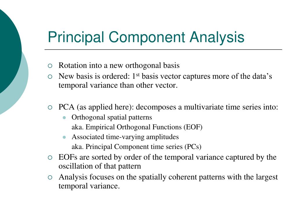
Principal Component Analysis. Rotation into a new orthogonal basis New basis is ordered: 1 st basis vector captures more of the data’s temporal variance than other vector. PCA (as applied here): decomposes a multivariate time series into: Orthogonal spatial patterns
Principal Component Analysis - slide 1
01 / 11Principal Component Analysis
1 / 17

Télécharger la présentation

Principal Component Analysis
Une image / un lien ci-dessous est fourni (tel quel) pour télécharger la présentation

Politique de téléchargement : le contenu du site vous est fourni TEL QUEL pour votre information et votre usage personnel ; il ne peut être vendu, concédé sous licence ni partagé sur d’autres sites sans l’accord de son auteur.Le contenu vous est fourni TEL QUEL, pour votre information et votre usage personnel uniquement. Téléchargez la présentation en cliquant sur ce lien. Lors du téléchargement, si vous ne parvenez pas à télécharger une présentation, l’éditeur a peut-être supprimé le fichier de son serveur.Pendant le téléchargement, si vous ne parvenez pas à obtenir une présentation, le fichier a peut-être été supprimé par l’éditeur.

F I N

Plus de contenu associé

Transcription de la présentation
  1. Principal Component Analysis • Rotation into a new orthogonal basis • New basis is ordered: 1st basis vector captures more of the data’s temporal variance than other vector. • PCA (as applied here): decomposes a multivariate time series into: • Orthogonal spatial patterns aka. Empirical Orthogonal Functions (EOF) • Associated time-varying amplitudes aka. Principal Component time series (PCs) • EOFs are sorted by order of the temporal variance captured by the oscillation of that pattern • Analysis focuses on the spatially coherent patterns with the largest temporal variance.

  2. PCA: 2 variable example Weakly Correlated Variables Strongly Correlated Variables

  3. PCA algorithm

  4. PCA algorithm, cont.

  5. PCA algorithm, cont.

  6. Features of PCA • EOFs must be mutually orthogonal; but physical modes need not be. • Leads to mode-mixing, particularly in higher EOFs • Decomposition is linear. • PCA does not utilize ordered data (time), the data is considered to be a unordered set of observations; so the temporal order can be used to provide further analysis after performing the PCA. • PCA are often calculated by an SVD of the centered data: EOFs (PCs) are proportional to the right (left) eigenvectors sorted by decreasing singular value.

  7. MOD EOF patterns and PC time series Var. (Cumul. Var.) Amplitude Spectra EOFs PCs 42% 33% (75%) 15% (90%) 3% (93%)

  8. MOD EOF 1: QBO (and Decadal) <= 0 R=0.80 ( 1% ) Captures 42% of the interannual variance.

  9. EOF 4: ENSO <= 0 R=0.71 ( < 0.1% ) Captures 3% of the interannual variance.

  10. PCA revisited • Eigenvectors (spatial patterns) can be thought of as empirically derived normal modes. • PC time series are the time-varying amplitudes of each mode: like a drum head. • Truncated PCA is a good way to reduce the data set to subspace – least variability lost. • Recent work developing nonlinear PCA techniques (e.g., Monahan & Fyfe – Neural Networks to find a lower dimensional manifold)

  11. NCEP Geopotential Height:30mb – 100mb Layer thickness Cumul. Var Amplitude Spectra EOFs PCs 79% R=0.43 ( > 15% ) 93% R=0.92 ( < 0.01% ) R=0.82 ( << 0.01%) 96% 97%