Download
1 / 39
390 likes | 496 Vues
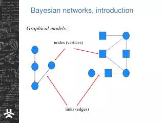
Learn about Bayesian Networks and plausible reasoning, including examples, dependencies, and conditional probabilities. Explore the three major models of probability and their derivations.

E N D
An Introduction to Bayesian Networks January 10, 2006 Marco Valtorta SWRG 3A55 mgv@cse.sc.edu
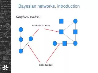
Uncertainty in Artificial Intelligence • Artificial Intelligence (AI) • [Robotics] • Automated Reasoning • [Theorem Proving, Search, etc.] • Reasoning Under Uncertainty • [Fuzzy Logic, Possibility Theory, etc.] • Normative Systems • Bayesian Networks • Influence Diagrams (Decision Networks)
Plausible Reasoning • Examples: • Icy Roads • Earthquake • Holmes’s Lawn • Car Start • Patterns of Plausible Reasoning • Serial (head-to-tail), diverging (tail-to-tail) and converging (head-to-head) connections • D-separation • The graphoid axioms
Requirements • Handling of bidirectional inference • Evidential and causal inference • Inter-causal reasoning • Locality (“regardless of anything else”) and detachment (“regardless of how it was derived”) do not hold in plausible reasoning • Compositional (rule-based, truth-functional approaches) are inadequate • Example: Chernobyl
Dependencies • In the better model, ThousandDead is independent of the Reports given PhoneInterview. We can safely ignore the reports, if we know the outcome of the interview. • In the naïve Bayes model, RadioReport is necessarily independent of TVReport, given ThousandDead. This is not true in the better model. • Therefore, the naïve Bayes model cannot simulate the better model.
Probabilities Let Ω be a set of sample points, F be a set of events relative to Ω, and P a function that assigns a unique real number to each E in F . Suppose that • P(E) >= 0 for all E in F • P(Ω) = 1 • If E1 and E2 are disjoint subsets of F , then P(E1 V E2) = P(E1) + P(E2). Then, the triple (Ω, F ,P) is called a probability space, and P is called a probability measure on F .
Conditional probabilities • Let (Ω, F ,P) be a probability space and E1 in F such that P(E1) > 0. Then for E2 in F , the conditional probability of E2 given E1, which is denoted by P(E2| E1), is defined as follows:
Models of the Axioms • There are three major models (i.e., interpretations in which the axioms are true) of the axioms of Kolmogorov and of the definition of conditional probability. • The classical approach • The limiting frequency approach • The subjective (Bayesian) approach
Derivation of Kolmogorov’s Axioms in the Classical Approach Let n be the number of equipossible outcomes in Ω If m is the number of equipossible outcomes in E, then P(E) = m/n ≥0 P(Ω) = n/n = 1 Let E1 and E2 be disjoint events, with m equipossible outcomes in E1 and k equipossible outcomes in E2. Since E1 and E2 are disjoint, there are k+m equipossible outcomes in E1 V E2, and: P(E1)+P(E2) = m/n + k/n = (k+m)/n = P(E1 V E2)
Conditional Probability in the Classical Approach • Let n, m, k be the number of sample points in Ω, E1, and E1&E2. Assuming that the alternatives in E1 remain equipossible when it is known that E1 has occurred, the probability of E2 given that E1 has occurred, P(E2|E1), is: k/m = (k/n)/(m/n) = P(E1&E2)/P(E1) • This is a theorem that relates unconditional probability to conditional probability.
The Subjective Approach • The probability P(E) of an event E is the fraction of a whole unit value which one would feel is the fair amount to exchange for the promise that one would receive a whole unit of value if E turns out to be true and zero units if E turns out to be false • The probability P(E) of an event E is the fraction of red balls in an urn containing red and brown balls such that one would feel indifferent between the statement "E will occur" and "a red ball would be extracted from the urn."
The Subjective Approach II • If there are n mutually exclusive and exhaustive events Ei, and a person assigned probability P(Ei) to each of them respectively, then he would agree that all n exchanges are fair and therefore agree that it is fair to exchange the sum of the probabilities of all events for 1 unit. Thus if the sum of the probabilities of the whole sample space were not one, the probabilities would be incoherent. • De Finetti derived Kolmogorov’s axioms and the definition of conditional probability from the first definition on the previous slide and the assumption of coherency.
Definition of Conditional Probability in the Subjective Approach • Let E and H be events. The conditional probability of E given H, denoted P(E|H), is defined as follows: Once it is learned that H occurs for certain, P(E|H) is the fair amount one would exchange for the promise that one would receive a whole unit value if E turns out to be true and zero units if E turns out to be false. [Neapolitan, 1990] • Note that this is a conditional definition: we do not care about what happens when H is false.
Derivation of Conditional Probability • One would exchange P(H) units for the promise to receive 1 unit if H occurs, 0 units otherwise; therefore, by multiplication of payoffs: • One would exchange P(H)P(E|H) units for the promise to receive P(E|H) units if H occurs, 0 units if H does not occur (bet 1); furthermore, by definition of P(E|H), if H does occur: • One would exchange P(E|H) units for the promise to receive 1 unit if E occurs, and 0 units if E does not occur (bet 2) • Therefore, one would exchange P(H)P(E|H) units for the promise to receive 1 unit if both H and E occur, and 0 units otherwise (bet 3). • But bet 3 is the same that one would accept for P(E&H), i.e. one would exchange P(E&H) units for the promise to receive 1 unit if both H and E occur, and 0 otherwise, and therefore P(H)P(E|H)=P(E&H).
Probability Theory as a Logic of Plausible Inference • Formal Justification: • Bayesian networks admit d-separation • Cox’s Theorem • Dutch Books • Dawid’s Theorem • Exchangeability • Growing Body of Successful Applications
Visit to Asia Example • Shortness of breadth (dyspnoea) may be due to tuberculosis, lung cancer or bronchitis, or none of them, or more than one of them. A recent visit to Asia increases the chances of tuberculosis, while smoking is known to be a risk factor for both lung cancer and bronchitis. The results of a single chest X-ray do not discriminate between lung cancer and tuberculosis, as neither does the presence of dyspnoea [Lauritzen and Spiegelhalter, 1988].
Visit to Asia Example • Tuberculosis and lung cancer can cause shortness of breadth (dyspnea) with equal likelihood. The same is true for a positive chest Xray (i.e., a positive chest Xray is also equally likely given either tuberculosis or lung cancer). Bronchitis is another cause of dyspnea. A recent visit to Asia increases the likelihood of tuberculosis, while smoking is a possible cause of both lung cancer and bronchitis [Neapolitan, 1990].
α τ ε λ σ β δ ξ Visit to Asia Example α (Asia): P(a)=.01 ε (λ or β):P(e|l,t)=1 P(e|l,~t)=1 τ (TB): P(t|a)=.05 P(e|~l,t)=1 P(t|~a)=.01 P(e|~l,~t)=0 σ(Smoking): P(s)=.5 ξ: P(x|e)=.98 P(x|~e)=.05 λ(Lung cancer): P(l|s)=.1 P(l|~s)=.01 δ (Dyspnea): P(d|e,b)=.9 P(d|e,~b)=.7 β(Bronchitis): P(b|s)=.6 P(d|~e.b)=.8 P(b|~s)=.3 P(d|~e,~b)=.1
Three Computational Problems • For a Bayesian network, we presents algorithms for • Belief Assessment • Most Probable Explanation (MPE) • Maximum a posteriori Hypothesis (MAP)
Belief Assessment • Definition • The belief assessment task of Xk = xk is to find • In the Visit to Asia example, the belief assessment problem answers questions like • What is the probability that a person has tuberculosis, given that he/she has dyspnea and has visited Asia recently ? • where k – normalizing constant
Most Probable Explanation (MPE) • Definition • The MPE task is to find an assignment xo = (xo1, …, xon) such that • In the Visit to Asia example, the MPE problem answers questions like • What are the most probable values for allvariables such that a person doesn’t catch dyspnea ?
Maximum A posteriori Hypothesis (MAP) • Definition • Given a set of hypothesized variables A = {A1, …, Ak}, , the MAP taskis to find an assignment ao = (ao1, …, aok) such that • Inthe Visit to Asia example, the MAP problem answers questions like • What are the most probable values for a person having both lung cancerand bronchitis, given that he/she has dyspnea and that his/her X-ray is positive?
Comments on the Axioms • Madsen’s dissertation (section 3.1.1) after Shenoy and Shafer. The axioms are maybe best described in Shenoy, Prakash P. “Valuation-Based Systems for Discrete Optimization.” Uncertainty in Artificial Intelligence, 6 (P.P. Bonissone, M. Henrion, L.N. Kanal, eds.), pp.385-400. The first axioms is written in quite a different form in that reference, but Shenoy notes that his axiom “can be interpreted as saying that the order in which we delete the variables does not matter,” “if we regards marginalization as a reduction of a valuation by deleting variables.” This seems to be what Madsen emphasizes in his axiom 1. • Another key reference, with an abstract algebraic treatment is made, is S. Bistarelli, U. Montanari, and F. Rossi. “Semiring-Based Constraint Satisfaction and Optimization,” Journal of the ACM 44, 2 (March 1997), pp.201-236. The authors explicitly mention Shenoy’s axioms as a special case in section 5, where they also discuss the solution of the secondary problem of Non-Serial Dynamic Programming [Bertelè and Brioschi, 1972]. Finally, an alternative algebraic generalization is in: S.L. Lauritzen and F.V. Jensen, “Local Computations with Valuations from a Commutative Semigroup,” Annals of Mathematics and Artificial Intelligence 21 (1997), pp.51-69.
Some Algorithms for Belief Update • Construct joint first (not based on local computation) • Stochastic Simulation (not based on local computation) • Conditioning (not based on local computation) • Direct Computation • Variable elimination • Bucket elimination (described next), variable elimination proper, peeling • Combination of potentials • SPI, factor trees • Junction trees • L&S, Shafer-Shenoy, Hugin, Lazy propagation • Polynomials • Castillo et al., Darwiche
Ordering the Variables Method 1 (Minimum deficiency) Begin elimination with the node which adds the fewest number of edges 1. , , (nothing added) 2. (nothing added) 3. , , , (one edge added) Method 2 (Minimum degree) Begin elimination with the nodewhich has the lowest degree 1. , (degree = 1) 2. , , (degree = 2) 3. , , (degree = 2)
Elimination Algorithm for Belief Assessment P(| =“yes”, =“yes”) = X\ {} (P(|)* P(|)* P(|,)* P(|,)* P()*P(|)*P(|)*P()) Bucket : P(|)*P(), =“yes” Hn(u)=xnПji=1Ci(xn,usi) Bucket : P(|) Bucket : P(|,), =“yes” Bucket : P(|,) H(,) H() Bucket : P(|) H(,,) Bucket : P(|)*P() H(,,) Bucket : H(,) k-normalizing constant Bucket : H() H() *k P(| =“yes”, =“yes”)
Elimination Algorithm for Most Probable Explanation Finding MPE = max ,,,,,,, P(,,,,,,,) MPE= MAX{,,,,,,,} (P(|)* P(|)* P(|,)* P(|,)* P()*P(|)*P(|)*P()) Bucket : P(|)*P() Hn(u)=maxxn (ПxnFnC(xn|xpa)) Bucket : P(|) Bucket : P(|,), =“no” Bucket : P(|,) H(,) H() Bucket : P(|) H(,,) Bucket : P(|)*P() H(,,) Bucket : H(,) Bucket : H() H() MPE probability
Elimination Algorithm for Most Probable Explanation Forward part ’ = arg maxP(’|)*P() Bucket : P(|)*P() Bucket : P(|) ’ = arg maxP(|’) Bucket : P(|,), =“no” ’ = “no” Bucket : P(|,) H(,) H() ’ = arg maxP(|’,’)*H(,’)*H() Bucket : P(|) H(,,) ’ = arg maxP(|’)*H(’,,’) Bucket : P(|)*P() H(,,) ’ = arg maxP(’|)*P()* H(’,’,) Bucket : H(,) ’ = arg maxH(’,) Bucket : H() H() ’ = arg maxH()* H() Return: (’, ’, ’, ’, ’, ’, ’, ’)