Download
1 / 51
520 likes | 700 Vues
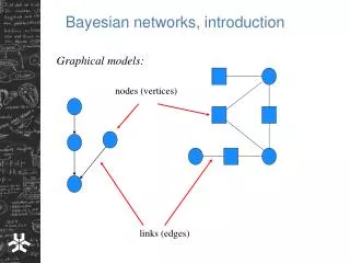
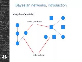
Bayesian networks, introduction. Graphical models:. nodes (vertices). links (edges). A graph can be disconnected: or connected: ; undirected : or directed:. the edges are one-directed arrows.

E N D
Bayesian networks, introduction Graphical models: nodes (vertices) links (edges)
A graph can be disconnected: or connected: ; undirected: or directed: the edges are one-directed arrows cyclic: or acyclic: possible to start in one node and “come back”
I2A F S I1 I2B BCE ABD A A B B C C BDG BEG D D E E DFG EGH F F G G H H Examples: Transport routes: Acyclic, but not completely directed Junction trees: From 8 nodes to 6 nodes (Source: Wikipedia)
Markov random field Given the light blue nodes, the middle blue node is conditionally independent of all other nodes (the white nodes)
Y X Bayesian (belief) networks • A Bayesian network is a connected directed acyclic graph (DAG) in which • the nodes represent random variables • the links represent direct relevance relationships among variables Examples: This small network has two nodes representing the random variable X and Y. The directed link gives a relevance relationship between the two variables that means Pr (Y = y | X = x, I ) Pr (Y = y | I )
Y X This network has three nodes representing the random variables X, Y and Z. The directed links give relevance relationships that means Pr ( Y = y | X = x, I ) Pr ( Y = y | I ) Pr ( Z = z | X = x, I ) Pr ( Z = z | I ) but also (as will be seen below) Pr ( Z = z | Y = y, X = x, I ) = Pr ( Z = z | X = x, I ) Z
Structures in a Bayesian network There are two classifications for nodes: parent nodes and child nodes parent node child node parent nodes Thus, a node can be solely a parent node, solely a child node or both! child nodes
Probability “tables” Each node represents a random variable. This random variable has either assigned probabilities (nominal scale or discrete) or an assigned probability density function (continuous scale) for its states. For a node that is solely a parent node: The assigned probabilities or density function are conditional on background information only (may be expressed as unconditional) For a node that is a child node (solely or joint parent/child): The assigned probabilities or density function are conditional on the states of its parent nodes (and on background information).
X Y Example: Probability tables X has the states x1 and x2 Y has the states y1 and y2
A? B? Example Dyes on banknotes (from previous lectures) Two states: Two states:
More about the structure… Ancestors and descendants: A node X is an ancestor of a node Y and Y is in turn a descendant of Xif there is a unidirectional path from X to Y A B C D E F G H I
Different connections: A diverging connection B C serial connection A B C A B converging connection C
Conditional independence and d-separation A 1) Diverging connection B C There is a path between B and C even if it not unidirectional B may be relevant for C (and vice versa) However, if the state of A is known this relevance is lost.: The path is blocked B and C are conditionally independent given A
Example: • Assume the old rat Willie was caught in a trap. • We have also found a sac with wheat grains with a small hole where grains have leaked out, and we suspect that Willie made this hole. • Examining the sac and Willie we find • traces of wheat grain in the jaw of Willie • traces of saliva at the damage on the sac that matches the DNA of Willie.
The whole scenario can be described with three random variables : A with the two states: A1: “Willie made the whole in the sac” A2: “Willie has not been near the sac” , B with the two states: B1: “Traces of wheat grain found in Willie’s jaw” B2: “No traces of wheat grain found in Willie’s jaw” , C with the two states: C1: “Match between saliva DNA and Willie’s DNA” C2: “No match in DNA between saliva and Willie” Note that the states of B and C are actually given, but the description gives a complete model
First we assume none of the states are given: Is B relevant for C ? Yes, because if B1 is true, i.e. we have found wheat grains in Willie’s jaw, the conditional probability of obtaining a match in DNA would be different from the corresponding conditional probability if B2 was true. Now assume for A that the state A2 is given, i.e. Willie was never near the sac. Under this condition B can no longer be relevant for C as whether we find a match in DNA between the saliva trace and Willie or not can have nothing to do with the grains we have found in Willie’s jaw. Now assume for A that the state A1 is given, i.e. Willie made the hole. Under this condition it is tempting to think that B is relevant for C, but the relevance is actually lost. Whether we find a match in DNA or not cannot have any impact on whether we find grains in the jaw or not once we have stated that Willie made the hole.
The scenario can be described with the Bayesian network A B C i.e. a diverging connection When a state of a node is assumed to be given we say the node is instantiated In the example, once A is instantiated the relevance relationship between B and C is lost. B and C are thus conditionally independent given a state of A
2) Serial connection There is a path between A and C (unidirectional from A to C) A may be relevant for C (and vice versa) If the state of B is known this relevance is lost.: The path is blocked A and C are conditionally independent given (a state of) B A B C
Example The Willie case with another description Let A be a random variable with states A1: “Willie made the hole in the sac” A2: “Willie did not make the hole” , B be a random variable with states B1: “Willie left saliva on the damage” B2: “Willie left no saliva” , C be a random variable with states C1: “There is a match in DNA” C2: “There is no match” Assuming no state is given, there is a relevance relationship between A and C:
Now assuming state B1 of B is given, i.e. we assume there was a contact between Willie’s jaw and the damage. A can no longer be relevant for C as once we have stated that Willie left saliva it does not matter for C whether he made the hole or not. The scenario can be described with the Bayesian network A B C Once B is instantiated the relevant relationship between A and C is lost. A and C are conditionally independent given a state of B
3) Converging connection There is a path between A and B (not unidirectional) A may be relevant for B (and vice versa) If the state of C is (completely) unknown this relevance does not exist. If the state of C is known (exactly or by a modification of the state probabilities) the path is opened A and C are conditionally dependent given information about the states of C, otherwise they are (conditionally) independent A B C
Example Paternity testing: child, mother and the true father Let A be a random variable representing the mother’s genotype in a specific locus B be a random variable representing the true father’s genotype in the same locus C be a random variable representing the child’s genotype in that locus A: A1 A2 B: B1 B2 C: C1 C2
If we know nothing about C (C1 and C2 are both unknown) , then • information about A cannot have any impact on B and vice versa. • If we on the other hand know the genotype of the child (C1 and C2 are both known or one of them is) then • knowledge of the genotype of the mother has impact on the probabilities of the different genotypes that can be possessed by the true father since the child must have inherited half of the genotype from the mother and the other half from the father. Bayesian network: A B C
d-separation • In a directed acyclic graph (DAG) the concept of d-separation is defined as: • Let SX, SY and SX be three disjoint subsets of variables included in the DAG • The sets SXand SY are d-separated given SZ if every path between a variable X in SX and a variable Y in SY contains • either • a serial connection through a variable Z in SZ or a divergent connection diverging from a variable Z in SZ • or • a converging connection converging to a variable Wnot inSZand of which no descendants belong to SX
X1 X2 Z2 Y1 Z1 Y3 Y2 Z3 • No direct link from red area to blue area or vice versa • No convergence from blue area and red area to green area W1 W2
The Markov property - formal definition of a Bayesian network Consider a variable X in a DAG Let PA(X ) be the set of all parents to X and DE(X ) be the set of all descendants to X. Let SY be a set of variables that does not include any variables in DE(X ), i.e. are not descendants of X Then, the DAG is a Bayesian network if and only if i.e. X is conditionally independent of SY given PA(X ) This is also known as the Markov property Note , by Pr(X | … ) we mean the probability of X having a particular state
Example Y1 Y2 Y4 Y3 W1 W2 X D1 D1 D3
Software • GeNIe (Graphical network Interface) • Software free-of-charge • Powerful for building complex network and running with moderately large probability tables • Download from http://genie.sis.pitt.edu/ • HUGIN • Commercial software • Probably today’s most powerful software for Bayesian networks • A demo version (less powerful than GeNIe) can be downloaded from www.hugin.com
Example A burglary was done in a shop. On the shop floor the police have secured a shoeprint. In the home of a suspect a shoe is found with a sole pattern that matches that of the shoeprint. In a compiled database of shoeprints it is found that the particular pattern is prevalent on 3 out of 657 prints. Hypotheses (usually called propositionsin forensic literature): Hp: “The shoeprint was made by the found shoe” Hd: “The shoeprint was made by some other shoe” “p” in Hp stands for “Prosecutor” (incriminating proposition) “d” in Hd stands for “Defence” (alternative to the incriminating) Evidence: E : “There is a match in pattern between shoeprint and the found shoe”
Setting the probability table for node E If proposition Hp(Shoeprint was made by found shoe) is true: If proposition Hd(Shoeprint was made by another shoe) is true: where is the proportion shoes in the (relevant) population of shoes having the observed pattern
The proportion is unknown, but an estimate from the database can be used
On the other we could directly have computed which is more accurate
Alternative network Propositions (as before): Hp: “The shoeprint was made by the found shoe” Hd: “The shoeprint was made by some other shoe” Evidence: X : Sole pattern of the found shoe States: q (the observed pattern) non-q Y : Pattern of the shoe print States: q non-q
H X Y in a network…
Note! We need to give a probability table for X to make the software work. However, we do not know but it does not matter what value we set here. Instantiate nodes X and Y both to q
Example: (more complex) In the head of the experienced examiner Assume there is a question whether an individual has a specific disease A or another disease B. What is observed is The individual has an increased level of substance 1 The individual has recurrent fever attacks The individual has light recurrent pain in the stomach
The experience of the examining physician says • If disease A is present it is quite common to have an increased level of substance 1. • If disease B is present it is less common to have an increased level of substance 1. • If disease A is present it is not generally common to have recurrent fever attacks, but if there is also an increased level of substance 1 such events are very common • Recurrent fever attacks are quite common when disease B is present regardless of the level of substance 1 • Recurrent pain in the stomach are generally more common when disease B is present than when disease A is present, and regardless of the level of substance 1 and whether fever attacks are present or not • If a patient has disease A, increased levels of substance 1 and recurrent fever attacks he/she would almost certainly have recurrent pain in the stomach. Otherwise, if disease A is present recurrent pain in the stomach is equally common. Can we put this up in a network?
Let the “disease node” be H, with states A and B Let the “evidence” nodes be X with states x1 :“The individual has an increased level of substance 1” x2 : “The individual has a normal level of substance 1” Y with states y1 :“The individual has recurrent fever attacks” y2 : “The individual has no fever attacks” Z with states z1 :“The individual has light recurrent pain in the stomach” z2 : “The individual has no pain in the stomach”
H X Y Z
The probabilities set out in the tables take into account some of the experience listed (e.g. that some probabilities are equal) However, we need to estimate numbers for , , , , , and Experience 1 & 2 >> Assume 0.8 and 0.2 Experience 3 high and < 0.5 Assume 0.9, 0.3 Experience 4 Assume 0.8 Experience 5 & 6 > Assume 0.6 and 0.4