Investment Appraisal and Real Options: Maximizing Shareholder Wealth

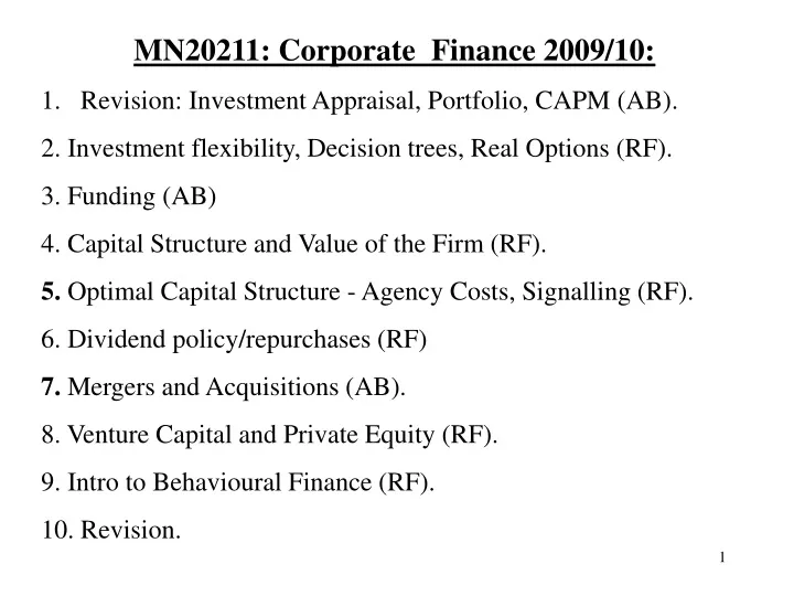
1. MN20211: Corporate Finance 2009/10: • Revision: Investment Appraisal, Portfolio, CAPM (AB). • 2. Investment flexibility, Decision trees, Real Options (RF). • 3. Funding (AB) • 4. Capital Structure and Value of the Firm (RF). • 5. Optimal Capital Structure - Agency Costs, Signalling (RF). • 6. Dividend policy/repurchases (RF) • 7. Mergers and Acquisitions (AB). • 8. Venture Capital and Private Equity (RF). • 9. Intro to Behavioural Finance (RF). • 10. Revision.

2. RF’s Lectures • Week 3: Investment flexibility/Real Options • Week 5: Capital Structure/Dividends • Week 6: Capital Structure/Dividends • Week 9: Venture Capital and Private Equity • Week 10: Introduction to BF/BCF. • Week 11 Revision

3. Lecture 3: Investment Flexibility/ Real options. • Reminder of Corporation’s Objective : Take projects that increase shareholder wealth (Value-adding projects). • Investment Appraisal Techniques: NPV, IRR, Payback, ARR • Decision trees • Monte Carlo. • Real Options

4. Lecture 3: Investment Flexibility, Decision Trees, and Real Options • Decision Trees and Sensitivity Analysis. • Example: From Ross, Westerfield and Jaffe: “Corporate Finance”. • New Project: Test and Development Phase: Investment $100m. • 0.75 chance of success. • If successful, Company can invest in full scale production, Investment $1500m. • Production will occur over next 5 years with the following cashflows.

5. Production Stage: Base Case Date 1 NPV = -1500 + = 1517

6. Decision Tree. Date 1: -1500 Date 0: -$100 NPV = 1517 Invest P=0.75 Success Do not Invest NPV = 0 Test Do not Invest Failure P=0.25 Do Not Test Invest NPV = -3611 Solve backwards: If the tests are successful, SEC should invest, since 1517 > 0. If tests are unsuccessful, SEC should not invest, since 0 > -3611.

7. Now move back to Stage 1. Invest $100m now to get 75% chance of $1517m one year later? Expected Payoff = 0.75 *1517 +0.25 *0 = 1138. NPV of testing at date 0 = -100 + = $890 Therefore, the firm should test the project. Sensitivity Analysis (What-if analysis or Bop analysis) Examines sensitivity of NPV to changes in underlying assumptions (on revenue, costs and cashflows).

8. Sensitivity Analysis. - NPV Calculation for all 3 possibilities of a single variable + expected forecast for all other variables. Limitation in just changing one variable at a time. Scenario Analysis- Change several variables together. Break - even analysis examines variability in forecasts. It determines the number of sales required to break even.

9. Real Options. A digression: Financial Options A call option gives the holder the right (but not the obligation) to buy shares at some time in the future at an exercise price agreed now. A put option gives the holder the right (but not the obligation) to sell shares at some time in the future at an exercise price agreed now. European Option – Exercised only at maturity date. American Option – Can be exercised at any time up to maturity. For simplicity, we focus on European Options.

10. Example: • Today, you buy a call option on Marks and Spencer’s shares. The call option gives you the right (but not the obligation) to buy MS shares at exercise date (say 31/12/10) at an exercise price given now (say £10). • At 31/12/10: MS share price becomes £12. Buy at £10: immediately sell at £12: profit £2. • Or: MS shares become £8 at 31/12/10: rip option up!

11. Factors Affecting Price of European Option (=c). • -Underlying Stock Price S. • -Exercise Price X. • Variance of of the returns of the underlying asset , • Time to maturity, T. The riskier the underlying returns, the greater the probability that the stock price will exceed the exercise price. The longer to maturity, the greater the probability that the stock price will exceed the exercise price.

12. Options: Payoff Profiles. Buying a Call Option. Selling a put option. Selling a Call Option. Buying a Put Option.

13. Pricing Call Options – Binomial Approach. Cu = 3 uS=24.00 q q c S=20 1- q 1- q dS=13.40 Cd=0 • S = £20. q=0.5. u=1.2. d=.67. X = £21. • 1 + rf = 1.1. • Risk free hedge Portfolio: Buy One Share of Stock and write m call options. • uS - mCu = dS – mCd => 24 – 3m = 13.40. • M = 3.53. By holding one share of stock, and selling 3.53 call options, your payoffs are the same in both states of nature (13.40): Risk free.

14. Since hedge portfolio is riskless: 1.1 ( 20 – 3.53C) = 13.40. Therefore, C = 2.21. This is the current price per call option. The total present value of investment = £12 .19, and the rate of return on investment is 13.40 / 12.19 = 1.1.

15. Alternative option-pricing method • Black-Scholes • Continuous Distribution of share returns (not binomial) • Continuous time (rather than discrete time).

16. Real Options • Just as financial options give the investor the right (but not obligation) to future share investment (flexibility) • Researchers recognised that investing in projects can be considered as ‘options’ (flexibility). • “Real Options”: Option to delay, option to expand, option to abandon. • Real options: dynamic approach (in contrast to static NPV).

17. Real Options • Based on the insights, methods and valuation of financial options which give you the right to invest in shares at a later date • RO: development of NPV to recognise corporation’s flexibility in investing in PROJECTS.

18. Real Options. • Real Options recognise flexibility in investment appraisal decision. • Standard NPV: static; “now or never”. • Real Option Approach: “Now or Later”. • -Option to delay, option to expand, option to abandon. • Analogy with financial options.

19. Types of Real Option • Option to Delay (Timing Option). • Option to Expand (eg R and D). • Option to Abandon.

20. Option to Delay (= call option) Value-creation Project value Investment in waiting: (sunk)

21. Option to expand (= call option) Value creation Project value Investment in initial project: eg R and D (sunk)

22. Option to Abandon ( = put option) Project goes badly: abandon for liquidation value. Project value

23. Valuation of Real Options • Binomial Pricing Model • Black-Scholes formula

24. Value of a Real Option • A Project’s Value-added = Standard NPV plus the Real Option Value. • For given cashflows, standard NPV decreases with risk (why?). • But Real Option Value increases with risk. • R and D very risky: => Real Option element may be high.

25. Simplified Examples • Option to Expand (page 241 of RWJ) If Successful Expand Build First Ice Hotel Do not Expand If unsuccessful

26. Option to Expand (Continued) • NPV of single ice hotel • NPV = - 12,000,000 + 2,000,000/0.20 =-2m • Reject? • Optimistic forecast: NPV = - 12M + 3M/0.2 • = 3M. • Pessimistic: NPV = -12M + 1M/0.2 = - 7m • Still reject?

27. Option to expand (continued) • Given success, the E will expand to 10 hotels • => • NPV = 50% x 10 x 3m + 50% x (-7m) = 11.5 m. • Therefore, invest.

28. Option to abandon. • NPV(opt) = - 12m + 6m/0.2 = 18m. • NPV (pess) = -12m – 2m/0.2 = -22m. • => NPV = - 2m. Reject? • But abandon if failure => • NPV = 50% x 18m + 50% x -12m/1.20 • = 2.17m • Accept.

29. Option to delay and Competition (Smit and Ankum). • -Smit and Ankum present a binomial real option model: • Option to delay increases value (wait to observe market demand) • But delay invites product market competition: reduces value (lost monopoly advantage). • cost: Lost cash flows • Trade-off: when to exercise real option (ie when to delay and when to invest in project). • Protecting Economic Rent: Innovation, barriers to entry, product differentiation, patents. • Firm needs too identify extent of competitive advantage.

30. Option to delay versus competition: Game-theoretic approach

31. Option to delay versus competition: effects of legal system

32. Monte Carlo methods • BBQ grills example in RWJ. • Application to Qinetiq (article by Tony Bishop).

33. Use of Real Options in Practice

34. Lecture 5 and 6: Capital Structure and Dividends. Positive NPV project immediately increases current equity value (share price immediately goes up!) Pre-project announcement New capital (all equity) New project: Value of Debt Original equity holders New equity New Firm Value

35. Example: =500+500=1000. 20 60 -20 = 40. Value of Debt = 500. Original Equity = 500+40 = 540 New Equity = 20 =1000+60=1060. Total Firm Value

36. Positive NPV: Effect on share price. Assume all equity.

37. Value of the Firm and Capital Structure Value of the Firm = Value of Debt + Value of Equity = discounted value of future cashflows available to the providers of capital. (where values refer to market values). Capital Structure is the amount of debt and equity: It is the way a firm finances its investments. Unlevered firm = all-equity. Levered firm = Debt plus equity. Miller-Modigliani said that it does not matter how you split the cake between debt and equity, the value of the firm is unchanged (Irrelevance Theorem).

38. Value of the Firm = discounted value of future cashflows available to the providers of capital. -Assume Incomes are perpetuities. Miller- Modigliani Theorem: Irrelevance Theorem: Without Tax, Firm Value is independent of the Capital Structure. Note that

39. K Without Taxes K With Taxes D/E D/E V V D/E D/E

40. Examples • Firm X • Henderson Case study

41. MM main assumptions: • - Symmetric information. • Managers unselfish- maximise shareholders wealth. • Risk Free Debt. • MM assumed that investment and financing decisions were separate. Firm first chooses its investment projects (NPV rule), then decides on its capital structure. • Pie Model of the Firm: D E E

42. MM irrelevance theorem- firm can use any mix of debt and equity – this is unsatisfactory as a policy tool. Searching for the Optimal Capital Structure. -Tax benefits of debt. -Asymmetric information- Signalling. -Agency Costs (selfish managers). -Debt Capacity and Risky Debt. Optimal Capital Structure maximises firm value.

43. Combining Tax Relief and Debt Capacity (Traditional View). K V D/E D/E

44. Section 4: Optimal Capital Structure, Agency Costs, and Signalling. Agency costs - manager’s self interested actions. Signalling - related to managerial type. Debt and Equity can affect Firm Value because: - Debt increases managers’ share of equity. -Debt has threat of bankruptcy if manager shirks. - Debt can reduce free cashflow. But- Debt - excessive risk taking.

45. AGENCY COST MODELS. Jensen and Meckling (1976). - self-interested manager - monetary rewards V private benefits. - issues debt and equity. Issuing equity => lower share of firm’s profits for manager => he takes more perks => firm value Issuing debt => he owns more equity => he takes less perks => firm value

46. Jensen and Meckling (1976) V Slope = -1 V* A V1 B1 B If manager owns all of the equity, equilibrium point A.

47. Jensen and Meckling (1976) V Slope = -1 V* A B V1 Slope = -1/2 B1 B If manager owns all of the equity, equilibrium point A. If manager owns half of the equity, he will got to point B if he can.

48. Jensen and Meckling (1976) V Slope = -1 V* A B V1 Slope = -1/2 V2 C B1 B2 B If manager owns all of the equity, equilibrium point A. If manager owns half of the equity, he will got to point B if he can. Final equilibrium, point C: value V2, and private benefits B1.

49. Jensen and Meckling - Numerical Example. Manager issues 100% Debt. Chooses Project B. Manager issues some Debt and Equity. Chooses Project A. Optimal Solution: Issue Debt?

50. Issuing debt increases the manager’s fractional ownership => Firm value rises. -But: Debt and risk-shifting.