Story of Machine Learning

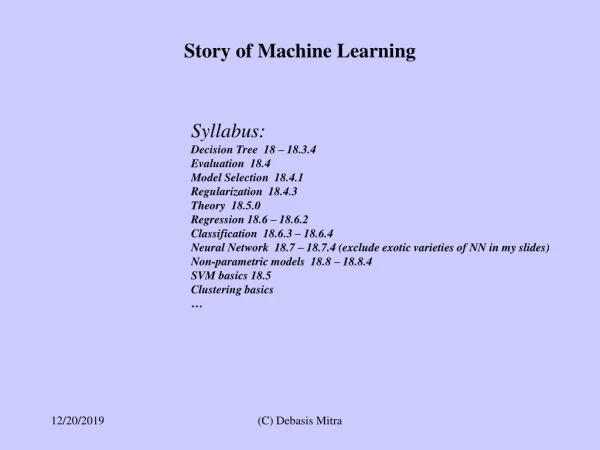
1. Story of Machine Learning Syllabus: Decision Tree 18 – 18.3.4 Evaluation 18.4 Model Selection 18.4.1 Regularization 18.4.3 Theory 18.5.0 Regression 18.6 – 18.6.2 Classification 18.6.3 – 18.6.4 Neural Network 18.7 – 18.7.4 (exclude exotic varieties of NN in my slides) Non-parametric models 18.8 – 18.8.4 SVM basics 18.5 Clustering basics … (C) Debasis Mitra

2. INFORMATION ENTROPY: If one were to transmit sequences comprising the 4 characters 'A', 'B', 'C', and 'D', a transmitted message might be 'ABADDCAB'. Information theory gives a way of calculating the smallest possible amount of information that will convey this. If all 4 letters are equally likely (25%), one can't do better (over a binary channel) than to have 2 bits encode (in binary) each letter: 'A' might code as '00', 'B' as '01', 'C' as '10', and 'D' as '11'. If 'A' occurs with 70% probability, 'B' with 26%, and 'C' and 'D' with 2% each, and could assign variable length codes, so that receiving a '1' says to look at another bit unless 2 bits of sequential 1s have already been received. In this case, 'A' would be coded as '0' (one bit), 'B' as '10', and 'C' and 'D' as '110' and '111'. It is easy to see that 70% of the time only one bit needs to be sent, 26% of the time two bits, and only 4% of the time 3 bits. On average, fewer than 2 bits are required since the entropyis lower (owing to the high prevalence of 'A' followed by 'B' – together 96% of characters). The calculation of the sum of weighted log probabilities measures and captures this effect. https://en.wikipedia.org/wiki/Entropy_(information_theory) (C) Debasis Mitra

3. Decision Tree: Choice of attribute at each level Entropy of Target Examples (current level): H(Goal) = P(vk) ∑k log2 (1/P(vk)), k may be {True, False} Say, 8 positive examples, and 4 negative examples H(Goal) = B(8/12)= (8/12) log2 (12/8) + (4/12) log2 (12/4) Now, for attribute A, calculate entropy: but say, attribute A has three values {some, full, none} Say, vs, vf, vn are number of examples for these three types, and (ps, ns) are positive and negative examples for the Target-label attribute (to go to restaurant or not) such that ps + ns = vs , and so are for (pf, nf) , (pn, nn) (C) Debasis Mitra

4. Decision Tree: Choice of attribute at each level Now, for attribute A, calculate entropy: but say, attribute A has three values {some, full, none} Say, vs, vf, vn are number of examples for these three types, and (ps, ns) are positive and negative examples for the Target attribute (to go to restaurant or not) such that ps + ns = vs , and so are (pf, nf) , (pn, nn) Entropy, R(A) = (vs/total)[(ps/vs)log2(ps/vs)+ (ns/vs)log2(ns/vs)] + (vf/total)[(pf/vf)log2(ps/vs)+ (nf/vf)log2(nf/vf)] + the same for A=“none” total = vs + vf + vn (C) Debasis Mitra

5. Decision Tree: Choice of attribute at each level Now, for choosing attribute A, information gain will be Gain(A) = H(Goal) – R(A) Compute this gain for each attribute at the current level, Best attribute provides highest information gain (C) Debasis Mitra

6. Decision Tree: Choice of attribute at top level in the Restaurant example in book H(Goal), for 6 pos and 6 neg examples in total, =1 bit Gain(Patrons) = 1 – [(2/12)B(0/2) + (4/12)B(4/4) + (6/12)B(2/6)] = 0.541 bit Gain(Type) = 1 – [(2/12)B(1/2) + (2/12)B(1/2) + (4/12)B(2/4) + (4/12)B(2/4) = 0 bit B(q) is the entropy for a Boolean variable, with q=positives/total, B(q) = qlog2(1/q) + (1-q)log2(1/1-q) (C) Debasis Mitra

7. Machine Learning has two stages: Do not forget Stage 1: Training, with “known” data (in supervised learning: known labels) Stage 2: Inferencing (deploying trained ML model to its task: unknown input) Stage 2.1: Validating with “unknown” data to quantify how good the trained model is (C) Debasis Mitra

8. Evaluation of Algorithm Training set = Sample of real world Stationarity assumption: Real world has the same distribution as that of training data Independent and Identically distributed (iid): Each datum, training or in real world, has equal probability of appearing Non-stationarity or non-iid: data is changing over time, what you learned before is no longer useful (C) Debasis Mitra

9. Evaluation of Algorithm Cross-validation: divide data set into two groups - training and validation, for computing the rate of successful classification of test data. Measurement of validation: error rate on validation set An ML algorithm has many parameters: e.g., model (order of polynomial), learning rate, etc. Fine-tune those parameters using a WRAPPER algorithm, by repeated validation: need to repeat cross validation by randomly splitting the available data set. (C) Debasis Mitra

10. Evaluation of Algorithm k-fold Cross validation: 1/k part of data set is validation set, repeat x-number of times by randomly splitting 1/k k=n, for data set size n, is leave-one-out cross-validation Peeking: After k-fold cross-validation, ML algorithm may overfit known training data (if validation is over part of the training set) , but may not be as good for real life use (note: that may mean iid is not true) ML competitions hold out real test data, but still groups "cheat" by repeatedly submitting fine-tuned code. (C) Debasis Mitra

11. Model Selection Finding best hypothesis: two step process • Find best hypothesis space • Optimization to find the best hypothesis E.g., 1) Which order of polynomial, y=ax+b, or y = ax2 +bx +c? 2) Find a, b, c parameters values (C) Debasis Mitra

12. Regularization Optimization function may embed simplicity of model, or any other relevant knowledge E.g., Cost(h) = Error + λ(complexity) Cost(h) = (y – [… ax +b])2 + λ(number of parameters,=2 here, or a+b+…) • h is hypothesis, the polynomial • Cost(h) is the error to be minimized • Polynomial embedded may be of arbitrary order • λ is tunable regularization constant or hyper-parameter • (a+b+…) regularization term, lower the better h* = argmin{a,b, …} Cost(h), is to find parameters a, b, … (C) Debasis Mitra

13. Computational Learning Theory PAC learning – quality of an algorithm: Any seriously wrong hypothesis may be quickly found out with only a few examples Conversely, any hypothesis that survives after many examples is likely to be correct Provably Approximately Correct (PAC) learning algorithm (C) Debasis Mitra

14. Computational Learning Theory CLT provides a measure on PAC learning How many examples can make it - how accurate? Sample complexity is studied here If you want ε–accurate you need f(ε) number of samples, as CLT tries to find the function f(.) (C) Debasis Mitra

15. Problem II: Linear Regression (C) Debasis Mitra

16. Linear Regression Regression: Predicting a continuous value (e.g., y) out of input x values Least Square Error or L2-norm minimization Linear model, y = mx +b: Has closed form solution Eq 18.3 (C) Debasis Mitra

17. Linear Regression Loss(hw) = ∑j (yj – (w1xj + w0))2 , j goes over N data points Take partial derivatives over wi and equate each to zero, i goes over parameters. wis are parameters that the algorithm learns w1 = [N(∑jxjyj) – (∑jxj)(∑jyj)] / [N(∑jxj2) - (∑jxj)2 ] w0 = [∑jyj – w1(∑jxj)]] / N for two parameters (C) Debasis Mitra

18. Linear Regression Sometimes no solution is found in closed form (e.g., non-linear regression) Gradient Descent gets iteratively closer to the solution: determine the direction in each iteration and update w parameters above step-size may be updated in each iteration, a constant, or a fixed schedule Note: "direction" gets determined by the sign of error: +ve or -ve (useful in understanding classifier later) (C) Debasis Mitra

19. Multivariate Linear Regression Model is: y = w0 +w1x1 +w2x2 +..., for x1, x2, ...xnvariables in n-dimension Closed form solution is a matrix formulation with partial differential equations equated to 0 Gradient descent is: w start with arbitrary point in the parameter space (w vector); loop until convergence for each parameter wi in w do wi wi – α* ∂/∂wi(Loss(w) ); α is the step size or learning rate (C) Debasis Mitra

20. Multivariate Linear Regression Model is: y = w0 +w1x1 +w2x2 +..., for x1, x2, ...xnvariables Gradient descent update is: wi wi – α* ∂/∂wi (Loss(w) ); Loss function may be summed over all training examples For example, with 2 parameters: w0 w0 – α* ∑j(yj – hw(xj)); and w1 w1 – α* ∑j(yj – hw(xj))*xj … for all wi’s where hw(xj) is the predicted value for y (C) Debasis Mitra

21. Multivariate Linear Regression Loss function may be summed over all training examples For example, with 2 parameters: w0 w0 – α* ∑j(yj – hw(xj)); and w1 w1 – α* ∑j(yj – hw(xj))*xj …. Above update procedure is called batch-gradient descent Stochastic-gradient descent: For each training example j update all wis Typically, one uses a mix of the two: e.g., a fixed batch size (C) Debasis Mitra

22. Multivariate Linear Regression Loss function may be summed over all training examples For example, with 2 parameters for one variable data (yj = w0 + w1*xj): w0 w0 – α* ∑j(yj – hw(xj)); and w1 w1 – α* ∑j(yj – hw(xj))*xj Note, in multi-variate case, element of x is xij y = w0 +w1x1 +w2x2 +..., for i running over variables or parameters and, j running over training examples Update rule is Eq 18.6 w* = argminw ∑j L2(yj, w.xj) or, wi  wi + α* ∑j(yj – hwi(xj))*xij (C) Debasis Mitra

23. Multivariate Linear Regression Note: some dimensions may be irrelevant or of low importance: wi ~0 for some xi Attempt to eliminate irrelevant dimensions: use a penalty term in error function for "complexity" Loss(hw) = L2(hw) + ∑i |wi| L1 norm (absolute sum) is better for this second term on complexity of the model: "sparse model" : minimizes #of “dimensions” (Fig 18.14 p722) (C) Debasis Mitra

24. Problem III: LINEAR CLASSIFIER 18.6.3 • Predicting y is the objective for regression, but classifiers predicts “type” or “class” • The objective is to learn a Boolean function: hw(x) = 1 or 0: data point x is inthe class or not • Training problem: set of (x, y) is given, x are data points and now, y =1 or 0, find hw(x) that models y • Test / purpose: a data point x is given, predict if it is in the class or not (compute hw(x) ) (C) Debasis Mitra

25. LINEAR CLASSIFIER 18.6.3 • No longer hw(x) is the line expected to pass through (or close to) the data samples as in regression, but to separate or classify them into two sides of the line – in class or out of class • Model: w0 + w1x1 +w2x2 + ... ≥0, and hw(x) =1 if so, =0 otherwise • Finding the line is very similar as in regression: optimize for (w0, w1, …) (C) Debasis Mitra

26. LINEAR CLASSIFIER 18.6.3 • Rewrite the model: (w0, w1, w2, ...)T * (x0, x1, x2, ...) ≥0, a vector product where (…) is a column vector, (.)T stands for matrix transpose, and x0 = 1 • Consider two vectors, w= (w0, w1, w2, ...)T and x= (x0, x1, x2, ...)T • hw(x) = 1 when (w.x)≥0, otherwise hw(x) = 0 • Gradient descent (for linear separator) works as before. It is called: • Perceptron Learning rule: • wiwi +α*(y - hw(x) ) * xi, 0 ≤ i≤ n, updates from iteration to iteration • One can do Batchgradient descent (for-each w, inside for-each datum-loop) or • Stochastic gradient descent (for-each datum, inside for-each w) here • Note: y here is also Boolean: 1 or 0 in the "training" set (C) Debasis Mitra

27. LINEAR CLASSIFIER 18.6.3 • Training: • (1) w stays same for correct prediction y= hw(x), • (2) False negative: y=1, but hw(x) =0, increase wi for each positive?(xi), decrease otherwise • (3) False positive: y=0, but hw(x) =1, decrease wi for each positive?(xi), increase otherwise (C) Debasis Mitra

28. LINEAR CLASSIFIER 18.6.3 • Logistic regression: use sigmoid hw(x) rather than Boolean function (step function) as above hw(x) = Logistic(w.x) = 1 / [1 + e-w.x] (C) Debasis Mitra

29. LINEAR CLASSIFIER 18.6.3 • Logistic regression: use sigmoid hw(x) rather than Boolean function (step function) as above hw(x) = Logistic(w.x) = 1 / [1 + e-w.x] • Update rule with above logistic regression model: Eq 18.8 p727 wiwi +α*(y - hw(x) ) * hw(x) * (1- hw(x) ) * xi • Continuous valued hw(x) may be interpreted as probability of being in the class (C) Debasis Mitra

30. Problem IV: ARTIFICIAL NEURAL NETWORK Ch 18.7 • Single Perceptron, only a linear classifier, a neuron in the network 1 x1 w0 w1 x2 w2 ∫ ∑i=0n wixi 0 or 1 xn wn (C) Debasis Mitra

31. ARTIFICIAL NEURAL NETWORK Ch 18.7 • A single layer perceptron network cannot "learn" xor function or Boolean sum, • Fig 18.21 p 730 (C) Debasis Mitra

32. ARTIFICIAL NEURAL NETWORK Ch 18.7 • Layers of perceptrons: Input  Hidden  Hidden  ...  Output classifying layer • Two essential components: Architecture, and Weights updating algorithm (C) Debasis Mitra

33. ARTIFICIAL NEURAL NETWORK Ch 18.7 • Perceptron output fed to multiple other perceptrons, Fig 18.19 p728 • Different types of hw(x) may be used, as activation function (C) Debasis Mitra

34. ARTIFICIAL NEURAL NETWORK Ch 18.7 • A single layer perceptron network cannot "learn" xor function or Boolean sum • Multi-layer Feed Forward Network: • Multiple layers can coordinate to create complex multi-linear classification space, • Fig 18.23 p732 (C) Debasis Mitra

35. ARTIFICIAL NEURAL NETWORK Ch 18.7 • Types of architectures: • Feed-forward Network: simple Directed Acyclic Graph • Recurrent Network: feedback loop (C) Debasis Mitra

36. ARTIFICIAL NEURAL NETWORK Ch 18.7.4 • Back-propagate, draw how error propagates backward • get total error del_E, weighted distribution over each backward nodes, • each node now knows its "errors“ or E’s, propagate that error recursively backward • all the way through input layer, • update weights or w’s (C) Debasis Mitra

37. ARTIFICIAL NEURAL NETWORK Ch 18.7.4 • Total loss function at the output layer, k neurons: Loss(w) = ∑k (yk – hw)2 = ∑k (yk – ak)2 , ak being the output produced • This is to be minimized • Gradient of this loss function is to iteratively lower: ∑k del/del_w (yk – ak)2 • Weight updates: wij wij + α * aj * Delj • aj is output of the neuron, Delj weighted modified error incorporating the activation function’s effect (see Eq 18.8) • Error propagation Delj = g’(inj) ∑k (wjkDelk), where g’() derivative of activation, k is over next layer neurons (previous layer in backward direction) • An iteration of backprop learning: Propagate errors then update weight, layer by layer backwards: (C) Debasis Mitra

38. GENERATIVE NEURAL NETWORK Not only classification… Transformations: say, (x,y) goes to (2x,y) – a linear transformation that we want to learn Neural Net: https://medium.com/wwblog/transformation-in-neural-networks-cdf74cbd8da8

39. GENERATIVE NEURAL NETWORK • Add translations (Affine transformation): Neural Net: https://medium.com/wwblog/transformation-in-neural-networks-cdf74cbd8da8

40. GENERATIVE NEURAL NETWORK • For non-linear transformations use non-linear activation function: https://medium.com/wwblog/transformation-in-neural-networks-cdf74cbd8da8

41. GENERATIVE NEURAL NETWORK • Multi-layer generative network for non-linear transformation: https://medium.com/wwblog/transformation-in-neural-networks-cdf74cbd8da8

42. GENERATIVE NEURAL NETWORK • Fourier Transform (a linear transform): Discrete Fourier Transform Computation Using Neural Networks, Rosemarie Velik, Vienna University of Technology

43. GENERATIVE NEURAL NETWORK • NN for Fourier Transform: • Learning should attain weight values from training Discrete Fourier Transform Computation Using Neural Networks, Rosemarie Velik, Vienna University of Technology

44. CONVOLUTIONAL NEURAL NETWORK • Running window weighted mean = convolution • Weights are learned • Pooling: Pick up a value (e,g., max) from a window – reduce size https://ujjwalkarn.me/2016/08/11/intuitive-explanation-convnets/

45. RECURRENT NEURAL NETWORK • Feed back loops are provided in the network • Independent from error propagation (backprop learning, weight update) algorithm: https://www.researchgate.net/figure/Graph-of-a-recurrent-neural-network_fig3_234055140

46. RECURRENT NEURAL NETWORK • An exotic recurrent network:

47. NON-PARAMETRIC MODELS Ch 18.8 • Parametric learning: hw has w as parameters • Non-parametric = no “curve fitting” • Simplest: Table look up (Problem V) For a query find a closest data point and return • We still need a sense of “distance” between data points, e.g., Lp-norm Lp(xj, xq) = (∑ki (xji – xqi)p )1/p , i runs over dimension of space, xj and xq are two points in that space (C) Debasis Mitra

48. NON-PARAMETRIC MODELS Ch 18.8 • K-nearest neighbor look up (kNN): find k nearest neighboring example data instead of one, • and vote by their attribute values (Pure counting for Boolean attributes) • k is typically odd integer for this reason (Problem VII) • Fig. 18.26 p738, shows the “query-space”, • runs query for every point in the 2D space to check what the prediction will return for any point • Gray areas indicate prediction=dark circle and white areas indicate prediction=open circle (C) Debasis Mitra

49. NON-PARAMETRIC MODELS Ch 18.8 • A different version of kNN: fix a distance value d and vote by all data points within • Advantage: faster search, conventional kNN may need very expensive data organization (Note: this is a search problem, before query gets answered) • Disadvantage: there may be too few data points within d, e.g. zero data point or no datum • Curse of dimensionality: number of dimensions (attributes) >> number of data • Sparsely distributed data points • Search is slow (C) Debasis Mitra

50. NON-PARAMETRIC MODELS Ch 18.8 • An efficient data organization: k-d tree • k is dimension here • Balanced binary search tree over k-dimension, with median (on each dimension) as the splitting boundary (C) Debasis Mitra