Lecture Notes II- 2 Dynamic Games of Complete Information
360 likes | 741 Vues
Lecture Notes II- 2 Dynamic Games of Complete Information. Extensive Form Representation (Game tree) Subgame Perfect Nash Equilibrium Repeated Games Trigger Strategy. Dynamic Games of Complete Information. Dynamic game with complete information

Lecture Notes II- 2 Dynamic Games of Complete Information
E N D
Presentation Transcript
Lecture Notes II-2 Dynamic Games of Complete Information • Extensive Form Representation (Game tree) • Subgame Perfect Nash Equilibrium • Repeated Games • Trigger Strategy
Dynamic Games of Complete Information • Dynamic game with complete information • Sequential games in which the players’ payoff functions are common knowledge • Perfect (imperfect) information: For each move in the play of the game, the player with the move knows (doesn’t know) the full history of the play of the game so far
Dynamic Game of Complete and Perfect Information • Key features • (1) the moves occur in sequence • (2) all previous moves are observed before the next move is chosen • (3) the players’ playoff from each feasible combination of moves are common knowledge
Backwards Induction • A simple dynamic game of complete and perfect information • 1. Player 1 chooses an action a1 from the feasible set A1 • 2. Player 2 observes a1 and then chooses an action a2 from the feasible set A2 • Payoffs are u1(a1,a2) and u2(a1,a2)
Backwards Induction (cont’) • The player 2’s optimization problem in the second stage • Assume that for each a1 in A1, players’ optimization problem has a unique solution, denoted by R2(a1) . This player 2’s reaction (or best response) to player 1’s action • The player 1’s optimization problem in the first stage • Assume that this optimization problem for player 1 also has a unique solution denoted by a1* • We call (a1*,R2*(a1*)) the backwards induction outcome of this game
Extensive-Form Representation 1 L R 2 2 0 L’ R’ 1 L” R” 1 1 3 0 0 2 In the first stage, player 1 play the optimal action L
Example 1: Stackelberg Model of Duopoly • Timing of the game • (1) firm 1 chooses a quantity q1 • (2) firm 2 observes q1 then choose a quantity q2 • Demand function • P(Q)=a-Q, Q=q1+q2 • Profit function to firm i • π(qi,qj)=qi[P(Q)-c]
Example 1: Stackelberg Model of Duopoly (cont’) • In the second stage, firm 2’s reaction to an arbitrary quantity by firm 1 R2(q1) is given by solving • In the first stage, firm 1’s problem is to solve • Outcome and
Example 1: Stackelberg Model of Duopoly (cont’) • Compare with Nash equilibrium of the simultaneous Cournot game Decide simultaneously Decide sequentially
Example 1: Stackelberg Model of Duopoly (cont’) Decide simultaneously Decide sequentially In single-person decision theory, having more information can never make the decision worse off, In game theory, however, having more information can make a player worse off
Two-Stage Game of Complete but Imperfect Information • A two-stage game • Players 1 and 2 simultaneously choose actions a1 and a2 from feasible sets A1 and A2, respectively • Players 3 and 4 observe the outcome of the first stage, (a1,a2), and then simultaneously choose actions a3 and a4 from feasible sets A3 and A4, respectively • Payoffs are ui(a1,a2,a3,a4) for i=1,2,3,4
Two-Stage Game of Complete but Imperfect Information (cont’) • Backward induction • For any feasible outcome of the first-stage game, (a1,a2), the second–stage that remains between players 3 and 4 has a unique Nash equilibrium (a3*(a1,a2), a4*(a1,a2)) • Subgame-perfect outcome • Suppose (a1*,a2*) is the unique Nash equilibrium of simultaneous-move game of player 1 and player 2 • (a1*,a2*,a3*(a1*,a2*),a4*(a1*,a2*)) is called subgame-perfect outcome
Example 2: Tariffs and Imperfect International Competition • Two identical countries, denoted by i=1,2 • Each country has a government that chooses a tariff rate ti, a firm that produces output for both home consumption hi and export ei • If the total quantity on the market in country i is Qi, then the market-clearing price is Pi(Qi)=a-Qi, where Qi=hi+ej • The total cost of production for firm i is Ci(hi,ei)=c(hi+ei)
Example 2: Tariffs and Imperfect International Competition (cont’) • Timing of the game • First, the governments simultaneously choose tariff rates t1 and t2 • Second, the firms observe the tariff rates and simultaneously choose quantities for home consumption and for export (h1,e1) and (h2,e2) • Payoffs are profit to firm i and total welfare to government i • welfare =consumers’ surplus + firms’ profit +tariff revenue
Example 2: Tariffs and Imperfect International Competition (cont’) Firm i’s profit Government i’s payoff P Consumers’ surplus a a-Q P=a-Q Q Qi
Example 2: Tariffs and Imperfect International Competition (cont’) Firm i’s optimization problem
Example 2: Tariffs and Imperfect International Competition (cont’) Government i’s optimization problem Implication (Cournot’s model), higher consumers’ surplus (free trade)
Two-Stage Repeated Game Prisoner 2 Player 2 L2 R2 L2 R2 L1 L1 Player 1 Player 1 R1 R1 • The unique subgame-perfect outcome of the two-stage • Prisoners’ Dilemma is (L1,L2) in the first stage, followed • by (L1,L2) in the second stage • Cooperation, that is, (R1,R2) cannon be achieved in • either stage of the subgame-perfect outcome
Finitely Repeated Game • Definition • Given a stage game G, let G(T) denote the finitely repeated game in which G is played T times, with the outcomes of all proceeding plays observed before the next play begins. The playoffs for G(T) are simply the sum of the playoffs from the T stage games • Proposition • If the stage game G has a unique Nash equilibrium then, for any finite T, the repeated game G(T) has a unique subgame-perfect outcome: the Nash equilibrium of G is played in every stage
Finitely Repeated Game with Multiple Nash Equilibrium L2 M2 R2 Two Nash equilibria (L1,L2) and (R1,R2) L1 Suppose the players anticipate that (R1,R2) will be the second-stage outcome if the first stage outcome is (M1,M2), but that (L1,L2) will be the second-stage if any of the eight other first stage outcome occurs M1 R1 L2 M2 R2 L1 Three subgame perfect Nash outcomes ((L1,L2), (L1,L2)) with payoff (2,2) ((M1,M2), (R1,R2)) with payoff (7,7) ((R1,R2), (L1,L2)) with payoff (4,4) M1 R1
Finitely Repeated Game with Multiple Nash Equilibrium (cont’) • Cooperation can be achieved in the first stage of a subgame-perfect outcome of the repeated game • If G is a static game of complete information with multiple Nash equilibria then in which, for any t<T, there may be subgame-perfect outcome in stage t is not a Nash equilibrium of G • Implication: credible threats or promises about future behavior can influence current behavior
Infinitely Repeated Games • Present value: Given the discount factor δ, the present value of the infinite sequence of payoffs,π1 ,π2 ,π3,... is • Trigger strategy: player i cooperates until someone fails to cooperate, which triggers a switch to noncooperation forever after • Trigger strategy is Subgame perfect Nash equilibrium when δ is sufficiently large • Implication: even if the stage game has a unique Nash equilibrium, there may be subgame-perfect outcomes of the infinitely repeated game in which no stage’s outcome is a Nash equilibrium
Infinitely Repeated Games: Example Player 2 • Trigger strategy • Play Ri in the first stage. In the tth stage, if the outcome of all t-1 proceeding stages has been (R1,R2) then play Ri; otherwise, play Li L2 R2 L1 Player 1 R1
Infinitely Repeated Games in Example (cont’) Player 2 L2 R2 L1 Player 1 R1 If any player deviates If no player deviates ( Solve ) Condition for both players to play the trigger strategy (Nash equilibrium)
Infinitely Repeated Games in Example (cont’) Player 2 L2 R2 L1 Player 1 R1 • The trigger strategy is a subgame perfect Nash equilibrium (Proof) • The infinitely repeated game can be grouped into two classes: • (1) Subgame in which all the outcomes of earlier stages have been (R1,R2) • Again the trigger strategy, which is Nash equilibrium of the whole game • (2) Subgames in which the outcome of at least one earlier stage differs from (R1,R2) • Repeat the stage-game equilibrium (L1,L2),which is also Nash equilibrium of the whole game
Example 3: Collusion between Cournot Duopolists • Trigger strategy • Produce half monopoly quantity,qm/2, in the first period. In the tth period, produce qm/2 if both firms have produced qm/2 in each of the t-1 previous periods; otherwise, produce the Cournot quantity
Example 3: Collusion between Cournot Duopolists (cont’) Competition profit Collusion profit Deviation profit Solve FOC Condition for both producer to play trigger strategy
Example 4: Efficiency Wages • The firms induce workers to work hard by paying high wages and threatening to fire workers caught shirking (Shapiro and Stiglitz 1984) • Stage game • First, the firms offers the worker a wage w • Second, the worker accepts or rejects the firm’s offer • If the worker rejects w, then the worker becomes self-employed at wage w0 • If the worker accepts w, then the worker chooses either to supply effort (which entails disutility e) or to shirk (which entails no disutility)
Example 4: Efficiency Wages (cont’) • The worker’s effort decision is not observed by the firm, but the worker’s output is observed by both the firm and the worker • Output can be either high (y) or low (0) • If the worker supplies effort then output is sure to be high • If the worker shirks then output is high with probability p and low with probability 1-p • Low output is an incontrovertible sigh of shirking • Payoffs: Suppose the firm employs the worker at wage w • if the worker supplies effort and output is high, the playoff of the firm is y-w and playoff of the worker is w-e • Efficient employment • y-e>w0>py
Example 4: Efficiency Wages (cont’) • Subgame-perfect outcome • The firm offer w=0 and the worker chooses self-employment • The firms pays in advance, the worker has no incentive to supply effort • Trigger strategy as repeated-game incentives • The firm’s strategy: offer w=w* (w*>w0) in the first period, and in each subsequent period to offer w=w* provided that the history of play is high-wage, high-output, but to offer w=0, otherwise • The worker’s strategy: accept the firm’s offer if w>w0 (choosing self-employment otherwise) the history of play, is high-wage, high-output (shirking otherwise)
Example 4: Efficiency Wages (cont’) • If it is optimal for the worker to supply effort, then the present value of the worker’s payoff is • If it is optimal for the worker to shirk, then the (expected) present value of the worker’s payoffs is
Example 4: Efficiency Wages (cont’) • It is optimal for the worker to supply effort if • The firm’s strategy is a best response to the worker’s if • We assume , the SPNE implies
Homework #2 • Problem set • 6,8,11,15,17 (from Gibbons) • Due date • two weeks from current class meeting • Bonus credit • Propose new applications in the context of IT/IS or potential extensions from examples discussed
