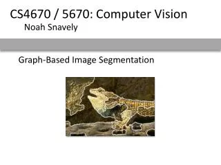
Graph-Based Segmentation
Graph-Based Segmentation. Readings: Szeliski , chapter5.4 5.4. http://www.cis.upenn.edu/~jshi/GraphTutorial/. Image segmentation. How do you pick the right segmentation?. Bottom up segmentation: - Tokens belong together because they are locally coherent. Top down segmentation:

Graph-Based Segmentation
E N D
Presentation Transcript
Graph-Based Segmentation Readings: Szeliski, chapter5.4 5.4 http://www.cis.upenn.edu/~jshi/GraphTutorial/
Image segmentation • How do you pick the right segmentation? • Bottom up segmentation: • - Tokens belong together because • they are locally coherent. • Top down segmentation: • - Tokens grouped because • they lie on the same object.
“Correct” segmentation • There may not be a single correct answer. • Partitioning is inherently hierarchical. • Presentation: • “Use the low-level coherence of brightness, color, texture or motion attributes to come up with partitions”
Affinity (Similarity) • Pixels in group A and B: high affinities • Connections between A, B: weak affinity • Cut
Normalized Cut • Cut Using a minimum cut usually involves isolating a single pixel
Normalized Cut Association within a cluster
Graph-based Image Segmentation G = {V,E} V: graph nodes E: edges connection nodes Pixels Pixel similarity Slides from Jianbo Shi
Graph terminology • Similarity matrix: Slides from Jianbo Shi
Affinity matrix N pixels Similarity of image pixels to selected pixel Brighter means more similar M pixels Warning the size of W is quadratic with the number of parameters! Reshape N*M pixels N*M pixels
Graph terminology • Degree of node: … … Slides from Jianbo Shi
Graph terminology • Volume of set: Association of A Slides from Jianbo Shi
Graph terminology • Cuts in a graph: Slides from Jianbo Shi
segments pixels Representation Partition matrix X: Pair-wise similarity matrix W: Degree matrix D: Laplacian matrix L: D=Diag(d)
Pixel similarity functions Intensity Distance Texture
Pixel similarity functions Intensity here c(x) is a vector of filter outputs. A natural thing to do is to square the outputs of a range of different filters at different scales and orientations, smooth the result, and rack these into a vector. Distance Texture
Definitions • Methods that use the spectrum of the affinity matrix to cluster are known as spectral clustering. • Normalized cuts, Average cuts, Average association make use of the eigenvectors of the affinity matrix. • Why these methods work?
Spectral Clustering Data Similarities * Slides from Dan Klein, Sep Kamvar, Chris Manning, Natural Language Group Stanford University
Eigenvectors and blocks • Block matrices have block eigenvectors: • Near-block matrices have near-block eigenvectors: 3= 0 1= 2 2= 2 4= 0 eigensolver 3= -0.02 1= 2.02 2= 2.02 4= -0.02 eigensolver * Slides from Dan Klein, Sep Kamvar, Chris Manning, Natural Language Group Stanford University
Spectral Space • Can put items into blocks by eigenvectors: • Clusters clear regardless of row ordering: e1 e2 e1 e2 e1 e2 e1 e2 * Slides from Dan Klein, Sep Kamvar, Chris Manning, Natural Language Group Stanford University
Outline • Graph terminology and representation. • “Min cuts” and “Normalized cuts”.
How do we extract a good cluster? • Simplest idea: we want a vector x giving the association between each element and a cluster • We want elements within this cluster to, on the whole, have strong affinity with one another • We could maximize • But need the constraint • This is an eigenvalue problem - choose the eigenvector of W with largest eigenvalue.
Cuts with lesser weight than the ideal cut Ideal Cut Minimum cut • Criterion for partition: A Problem! Weight of cut is directly proportional to the number of edges in the cut. B First proposed by Wu and Leahy
Normalized Cut Normalized cut or balanced cut: Finds better cut
Normalized Cut • Volume of set (or association): A B
Normalized Cut A • Volume of set (or association): • Define normalized cut: “a fraction of the total edge connections to all the nodes in the graph”: B A B • Define normalized association: “how tightly on average nodes within the cluster are connected to each other” A B
Observations(I) • Maximizing Nassoc is the same as minimizing Ncut, since they are related:
Algorithm • How to minimize Ncut? • Transform Ncut equation to a matricial form. • After simplifying: NP-Hard! y’s values are quantized Subject to: Rayleigh quotient
min Algorithm • Instead, relax into the continuous domain by solving generalized eigenvalue system: • Which gives: • Note that so, the first eigenvector is y0=1 with eigenvalue0. • The second smallest eigenvector is the real valued solution to this problem!!
Algorithm • Define a similarity function between 2 nodes. i.e.: • Compute affinity matrix (W) and degree matrix (D). • Solve • Use the eigenvector with the second smallest eigenvalue to bipartition the graph. • Decide if re-partition current partitions. Note: since precision requirements are low, W is very sparse and only few eigenvectors are required, the eigenvectors can be extracted very fast using Lanczos algorithm.
Algorithm Solve Normalized affinity matrix, (Weiss 1999)
Discretization • Sometimes there is not a clear threshold to binarize since eigenvectors take on continuous values. • How to choose the splitting point? • Pick a constant value (0, or 0.5). • Pick the median value as splitting point. • Look for the splitting point that has the minimum Ncutvalue: • Choose n possible splitting points. • Compute Ncut value. • Pick minimum.
Use k-eigenvectors • Recursive 2-way Ncut is slow. • We can use more eigenvectors to re-partition the graph, however: • Not all eigenvectors are useful for partition (degree of smoothness). • Procedure: compute k-means with a high k. Then follow one of these procedures: • Merge segments that minimize k-way Ncut criterion. • Use the k segments and find the partitions there using exhaustive search. • Compute Q (next slides). e1 e2 e1 e2
Toy examples Images from Matthew Brand (TR-2002-42)
Example (I) Eigenvectors Segments
Example (II) Original Segments * Slide from Khurram Hassan-Shafique CAP5415 Computer Vision 2003
Example (III) Comparative segmentation results (Alpert, Galun, Basri et al. 2007) probabilistic bottom-up merging
Segmentation Methods Using Eigenvectors • Graph terminology and representation. • “Min cuts” and “Normalized cuts”. • Other segmentation methods using eigenvectors.
Other Methods • Average association • Use the eigenvector of W associated to the biggest eigenvalue for partitioning. • Tries to maximize: • Has a bias to find tight clusters. Useful for gaussian distributions. A B
Other Methods • Average cut • Tries to minimize: • Very similar to normalized cuts. • We cannot ensure that partitions will have a tight within-group similarity since this equation does not have the nice properties of the equation of normalized cuts.
Other Methods Normalized cut Average cut 20 points are randomly distributed from 0.0 to 0.5 12 points are randomly distributed from 0.65 to 1.0 Average association
Other Methods Data W First ev Second ev Q • Scott and Longuet-Higgins (1990). • V contains the first k eigenvectors of W. • Normalize V by rows. • Compute Q=VTV • Values close to 1 belong to the same cluster.
Other Applications Data M Q • Costeira and Kanade (1995). • Used to segment points in motion. • Compute M=(XY). • The affinity matrix W is compute as W=MTM. This trick computes the affinity of every pair of points as a inner product. • Compute Q=VTV • Values close to 1 belong to the same cluster.