Graph-based Segmentation
Graph-based Segmentation. Main Ideas . Convert image into a graph Vertices for the pixels Edges between the pixels Additional vertices and edges to encode other constraints Manipulate the graph to segment the image. Papers.

Graph-based Segmentation
E N D
Presentation Transcript
Main Ideas • Convert image into a graph • Vertices for the pixels • Edges between the pixels • Additional vertices and edges to encode other constraints • Manipulate the graph to segment the image
Papers • Interactive graph cuts for optimal boundary & region segmentation ofobjects in N-D images • Boykov and Jolly • Minimize an energy function • Efficient Graph-based Segmentation • Felzenszwalb and Huttenlocher • Cluster the vertices based on edge weight
Boykov and Jolly • Binary image segmentation • Classify pixels as object or background • Their contribution is adding interactivity • Minimise an energy function • E(A) = B(A) + λR(A) • A: Segmentation (assign each pixels to object or background) • B(A): The cost of all the edges between object pixels and background pixels • R(A): The cost of deciding a pixel to be object or background
Creating the Graph • Each pixel has a corresponding vertex • Additionally, a source (“object”) and a sink (“background”) • Each pixel vertex has an edge to its neighbours (e.g. 8 adjacent neighbours in 2D), an edge to the source, an edge to the sink
Edge Weights between pixels • Weight of edges between pixel vertices are determined by the B() function • Low score when boundary is likely to pass between the vertices • high score when vertices are probably part of the same element • E.g. the difference in pixel intensities, the gradient
Edges to Source/Sink • If pixel is known to be an object, use a high weight (K) to the source, zero weight to the sink • K is chosen so that it will never be cut • Conversely, if pixel is background, use weight K to the sink, zero weight to the source • Otherwise, weigh edges to source and sink appropriately using the R() function • Note that the edge to the source is the “likelihood” for the pixel being the background – we break this edge when the pixel is assigned to the background
Applications • Handles arbitrary number of dimensions • Finds global minimum energy • Needs “good” user input to work effectively • Need intelligent functions • Need to select λ
Felzenszwalb and Huttenlocher • Download the program from the webpage: • http://people.cs.uchicago.edu/~pff/segment/ • Minimal documentation • Short README file • Paper
The program • Comes as a tar.gz archive and .zip archive • Process • Extract archive • ‘make’ (Makefile supplied) • Program consists of • A .cpp “wrapper” file (only calls the functions) • Actual algorithm functions are in .h files • Basic portable C++ code
Program Testing • Built on Mac OS X, Linux, Windows cygwin • Gcc toolchain, but any C++ compiler should work • Supplied basic Makefile • Results were basically the same between platforms • Colors are chosen randomly • Results obtained are not the same as posted on the website • Image files on the website may be modified (scaled/compressed/downsampled)
Algorithm • Create a graph • Each vertex corresponds to a vertex • Edges are between “neighbouring” vertices • Choose a small neighbourhood to reduce computation time (otherwise we have a complete graph) • Weight on the edge is the 5D distance between the points (for a 2D image) • 5D vector = x position, y position and 3 color components
Parameters • σ: Use this value and do Gaussian smoothing (preprocessing the image to reduce noise) • k: threshold value for doing the clustering • min: “hack” parameter • the smallest cluster size must contain at least this many vertices – clusters that are too small will be merged with other clusters until sufficiently large
Clustering • Put each vertex in a component • Sort edges by weight • Take each edge in turn • If the edge is between vertices in two different components A and B, we can merge if the edge weight is lower enough than the threshold • Threshold is the minimum of the following value, computed on A and B • (Lowest weight edge in minimum spanning tree of the component) + (k / size of component)
Notes • Low edge weights between vertices that are likely to be in the same cluster • As a cluster gets larger, it becomes harder to add vertices to it • Heuristic – not really minimising a particular energy function • More similar to “region growing” • User has select “good” parameters to get good results
Effect of σ • Increased smoothing results in removal of noise • Can cause “bleeding” – the algorithm has difficulty separating background from the object if the boundaries are too smooth
Increasing σ • Clouds are recognised as one object • Palm tree gets confused with ocean
Grain • Increasing σ introduces more blurring (reduces the edge weight between pixels)
Vertebrae MRI • Gets rid of noise (bottom left, right hand side), but purple vertebrate piece bleeds out
Increasing Threshold • Clusters more aggresively • Palm tree is confused with ocean and clouds
Grain • Non-grain pixels are almost all clustered together • Measure of how “similar” all the pixels of an object should be
MRI • Vertebrae and region next to vertebrae are very similar shade so are easily confused
Increasing ‘min’ value • Segmentation is the same, but small components are merged with neighboring ones
Grain • Easy to control change, gets rid of small artifacts
MRI • Not much effect if regions are already large
Parameter Tweaking • Need to manually tune parameters to get a good image • Image of MRI after selecting • σ = 0.6 • k = 200 • min = 60
Performance • Need to tune parameters by hand • Very fast • Program usually takes a couple seconds on the test images provided • Only takes ppm images in RAW data format • Theoretically, algorithm generalises to arbitrary number of dimensions and arbitrary number of features per pixel
Command-line tools • Working with images involves opening up the results in an image viewer – can get messy