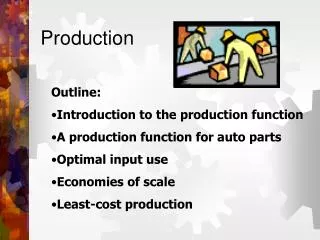
Production Functions in Economics
Learn about production functions, isoquants, total product curves, average & marginal products, and their relationship in economics. Study the law of diminishing returns and interpret curves to analyze productivity effectively.

Production Functions in Economics
E N D
Presentation Transcript
PRODUCTION • PRODUCTION FUNCTION: The term economists use to describe the technology of production, i.e., the relationship between inputs and the output of a good or service. Production
There is a production function for every good that shows the maximum output you can get from any quantities of inputs. The production function is the description of the current best technology for making a good. • Production functions apply to firms. E.g., MSU has a production function for producing alfalfa. GM has a production function for producing Chevy’s. Production
The next slide shows a production function when there are two variable inputs, L and K. Production
ISOQUANT • Definition: All combinations of inputs that yield the same output. • The isoquants for the production funtion in the last slide can be seen by viewing the function "from above". Production
Notice that isoquants seem to have many of the same properties as indifference curves. Production
TOTAL PRODUCT CURVE • The total product curve shows output as a function of a single variable input, holding all other inputs constant. Production
The production function for tax returns in a small accounting firm can be written like this: • Q(returns) = f(office space, accountants, computers, furniture, supervisors, office supplies, etc.) • The dependent variable is quantity of output (number of returns filed in this case). • The independent variables are quantities of inputs. Production
Here’s a table of values for tax return production as a function of a single variable input, LABOR: Total Labor Product 0 0 1 3 2 15 3 36 4 48 5 56 6 62 7 66 8 68 Production
Total product curve for tax returns as a function of the amount of labor Q 70 60 50 40 Plot the remaining points 30 20 10 0 0 1 2 3 4 5 6 7 8 9 10 LABOR Production
Average product: Output per unit of input, or (output / input). • APL = Q/L • Average product is a measure of input productivity. Production
If we know the total product curve for tax preparation services, we can compute the average product: TOTAL AVERAGE LABOR PRODUCT PRODUCT 0 0 1 3 3.00 2 15 7.50 15 / 2 3 36 12.00 4 48 5 56 11.20 56 / 5 6 62 7 66 8 68 8.50 Production
The average product curve shows the average product of an input as a function of the amount of input used. • The independent variable is the amount of the input (labor). • The dependent variable is the average product (of labor). Production
APL 22 The average product of 7 units of labor is 9.43. 20 • Graph the points showing AP, and connect them here. Label the axes correctly. 18 16 14 12 10 AP 8 6 4 2 0 0 2 4 6 8 10 LABOR Production
Marginal product of an input: The change in output per unit change in input. Marginal product is the slope of the total product curve: Q/ L Marginal product is a measure of input productivity. Production
Total Marginal Labor Product Product 0 0 1 3 3 2 15 12 (48-36)/ (4-3) 3 36 21 4 48 12 5 56 6 62 7 66 8 68
The marginal product curve shows the marginal product as a function of the quantity of labor used. • The independent variable is the amount of the input (labor). • The dependent variable is the marginal product of labor. Production
22 • Plot the remaining points showing MP here, and connect the them. Label the axes correctly. 20 18 16 14 12 10 8 6 4 2 0 0 2 4 6 8 10 Production
Q MP 80 22 TP The marginal product of the 6th unit of L is 6. 20 • Here’s a way to see the relationship between total product curve and the marginal product curve. 70 18 60 16 Q=6 50 14 12 L=1 40 10 30 Q / L 8 20 6 4 10 2 MP 0 L 0 L 0 1 2 3 4 5 6 7 8 9 10 0 2 4 6 8 10 Total Product Curve Marginal Product Curve Production
There is an important relationship between average product and marginal product of an input: • 1) When AP is rising, MP is greater than AP, • 2) When AP is falling, MP is less than AP. • 3) When AP is constant (neither rising nor falling), MP equals AP. Production
MP, AP 22 • So the average and marginal products must look like this: 20 18 16 14 12 10 AP 8 6 4 MP 2 0 L 0 2 4 6 8 10 Production
Law of Diminishing Returns • As the amount of an input increases, all other inputs being held constant, the marginal product of the input will eventually decline. Production
MP, AP Diminishing returns begin here with the 4th unit of labor. 22 20 18 16 14 12 10 AP 8 6 4 MP 2 0 L 0 2 4 6 8 10 Production
The general shapes of the average and marginal product curves can be deduced from the total product curve. Production
Q 80 TP 70 60 50 Total Product Curve 40 30 20 10 0 When the slope of the TP curve is increasing, MP is rising. When the slope of the TP curve is decreasing, MP is falling. L 0 1 2 3 4 5 6 7 8 9 10 MP 22 20 18 16 14 12 10 8 6 4 Marginal Product Curve 2 MP 0 L 0 2 4 6 8 10 Production
The shape of the average product curve also can be found by looking at the total product curve. Production
THE SLOPE OF A LINE FROM THE ORIGIN TO A POINT ON THE TP CURVE MEASURES AVERAGE PRODUCT. Q AP 80 TP 22 So this distance is 12 20 70 18 60 16 The slope of this line is 12 (36/3) 14 50 12 40 10 30 8 AP 6 20 4 10 2 0 0 L L 0 1 2 3 4 5 6 7 8 9 10 0 2 4 6 8 10 To find AP draw lines from the origin to points on the TP curve at different levels of L. Production
THE SLOPE OF A LINE FROM THE ORIGIN TO A POINT ON THE TP CURVE MEASURES AVERAGE PRODUCT. Q AP So this distance is 9.43 22 TP 80 20 70 18 60 16 The slope of this line is 9.43 (66/7) 14 50 12 40 10 8 30 AP 6 20 4 10 2 0 0 L L 0 2 4 6 8 10 0 1 2 3 4 5 6 7 8 9 10 To find AP draw lines from the origin to points on the TP curve at different levels of L. Production
So to find the matching set of AP and MP curves for any TP curve proceed as follows: • 1) Find the general shape of the MP curve by seeing what happens to the slope of the TP curve as input increases. • 2) Find the general shape of the AP curve by seeing what happens to the slopes of lines from the origin as input increases. • 3) Remember the correct relationships between the curves, and sketch the curves to follow the required relationships. Production
A few practice problems: Q • Find the corresponding MP and AP curves for each TP curve: TP input Production
Q TP input Production
Q TP input Production
EXTRA CREDIT !!! Q TP input Production