Effect Size Estimation
Effect Size Estimation. Why and How An Overview. Statistical Significance. Only tells you sample results unlikely were the null true. Null is usually that the effect size is absolutely zero. If power is high, the size of a significant effect could be trivial.

Effect Size Estimation
E N D
Presentation Transcript
Effect Size Estimation Why and How An Overview
Statistical Significance • Only tells you sample results unlikely were the null true. • Null is usually that the effect size is absolutely zero. • If power is high, the size of a significant effect could be trivial. • If power is low, a big effect could fail to be detected
Nonsignificant Results • Effect size estimates should be reported here too, especially when power was low. • Will help you and others determine whether or not it is worth the effort to repeat the research under conditions providing more power.
Comparing MeansStudent’s T Tests • Even with complex research, the most important questions can often be addressed by simple contrasts between means or sets of means. • Reporting strength of effect estimates for such contrasts can be very helpful.
Symbols • Different folks use different symbols. Here are those I shall use • d – the parameter, Cohen’s d. • g – the sample statistic, Hedges’ g -- ditto • Warning: Many journals use d to refer to the sample statistic.
One Sample • On SAT-Q, is µ for my students same as national average? • Point estimate does not indicate precision of estimation. • We need a confidence interval.
Constructing the Confidence Interval • Approximate method – find unstandardized CI, divide endpoints by sample SD. • OK with large sample sizes. • With small sample sizes should use an exact method. • Computer-intensive, iterative procedure, must estimate µ and σ.
Programs to Do It • SAS • SPSS • The mean math SAT of my undergraduate statistics students (M = 535, SD = 93.4) was significantly greater than the national norm (516), t(113) = 2.147, p = .034, g = .20. A 95% confidence interval for the mean runs from 517 to 552. A 95% confidence interval for d runs from .015 to .386.
Benchmarks for d • What would be a small effect in one context might be a large effect in another. • Cohen reluctantly provided these benchmarks for behavioral research • .2 = small, not trivial • .5 = medium • .8 = large
Reducing Error • Not satisfied with the width of the CI, .015 to .386 (trivial to small/medium)? • Get more data, or • Do any of the other things that increase power.
Why Standardize? • Statisticians argue about this. • If the unit of measure is meaningful (cm, $, ml), do not need to standardize. • Weight reduction intervention produced average loss of 17.3 pounds. • Residents of Mississippi average 17.3 points higher than national norm on measure of neo-fascist attitudes.
Bias in Effect Size Estimation • Lab research may result in over-estimation of the size of the effect in the natural world. • Sample Homogeneity • Extraneous Variable Control • Mean difference = 25 • Lab SD = 15, g = 1.67, whopper effect • Field SD = 100, g = .25, small effect
Programs • Will do all this for you and give you a CI. • Conf_Interval-d2.sas • CI-d-SPSS.zip • Confidence Intervals, Pooled and Separate Variances T
Example • Pooled t(86) = 3.267 t = 3.267 ; df = 86 ; n1 = 33 ; n2 = 55 ; g = t/sqrt(n1*n2/(n1+n2)); ncp_lower = TNONCT(t,df,.975); ncp_upper = TNONCT(t,df,.025); d_lower = ncp_lower*sqrt((n1+n2)/(n1*n2)); d_upper = ncp_upper*sqrt((n1+n2)/(n1*n2)); output; run; proc print; var g d_lower d_upper; run; Obs g d_lower d_upper 1 0.71937 0.27268 1.16212 Among Vermont school-children, girls’ GPA (M = 2.82, SD = .83, N = 33) was significantly higher than boys’ GPA (M = 2.24, SD = .81, N = 55), t(65.9) = 3.24, p = .002, g = .72. A 95% confidence interval for the difference between girls’ and boys’ mean GPA runs from .23 to .95 in raw score units and from .27 to 1.16 in standardized units. This is an almost large effect by Cohen’s guidelines.
Glass’ Delta • Use the control group SD rather than pooled SD as the standardizer. • When the control group SD is a better estimate of SD in the population of interest.
Point Biserial r • Simply correlate group membership with the scores on the outcome variable. • Or compute • For the regression Score = a + bGroup, b = difference in group means = .588. • standardized slope = This is a medium-sized effect by Cohen’s benchmarks. Hmmmm. It was large when we used g.
Eta-Squared • For two mean comparisons, this is simply the squared point biserial r. • Can be interpreted as a proportion of variance. • CI: Conf-Interval-R2-Regr.sas orCI-R2-SPSS.zip • For our data, 2 = .11, CI.95 = .017, .240. • Again, overestimation results from EV control. • 2
Cohen’s Benchmarks for and 2 • • .1 is small but not trivial (r2 = 1%) • .3 is medium (9%) • .5 is large (25%) • 2 • .01 (1%) is small but not trivial • .06 is medium • .14 is large • Note the inconsistency between these two sets of benchmarks.
Effect of n1/n2 on g and rpb • n1/n2 = 1 • M1 = 5.5, SD1 = 2.306, n1 = 20, • M2 = 7.8, SD2 = 2.306, n2 = 20 • t(38) = 3.155, p = .003 • M2-M1 = 2.30 g = 1.00 rpb = .456 • Large effect
Effect of n1/n2 on g and rpb • n1/n2 = 25 • M1 = 5.500, SD1 = 2.259, n1 = 100, • M2 = 7.775, SD2 = 2.241, n2 = 4 • t(102) = 1.976, p = .051 • M2-M1 = 2.30 g = 1.01 rpb = .192 • Large or (Small to Medium) Effect?
How does n1/n2 affect rpb? • The point biserial r is the standardized slope for predicting the outcome variable from the grouping variable (coded 1,2). • The unstandardized slope is the simple difference between group means. • Standardize by multiplying by the SD of the grouping variable and dividing by the SD of the outcome variable. • The SD of the grouping variable is a function of the sample sizes. For example, for N = 100, the SD of the grouping variable is • .503 when n1, n2 = 50, 50 • .473 when n1, n2 = 67, 33 • .302 when n1, n2 = 90, 10
Common Language Effect Size Statistic • Find the lower-tailed p for • For our data, p = .5, • If you were to randomly select one boy & one girl. P(Girl GPA > Boy GPA) = .69. • Odds = .69/(1-.69) = 2.23.
Two Related Samples • Treat the data as if they were from independent samples when calculating g. • If you standardize with the SD of the difference scores, you will overestimate d. • There is not available software to get an exact CI, and approximation procedures are only good with large data sets.
Correlation/Regression • Even in complex research, many questions of great interest are addressed by zero-order correlation coefficients. • Pearson r, are already standardized. • Cohen’s Benchmarks: • .1 = small, not trivial • .3 = medium • .5 = large
CI for , Correlation Model • All variables random rather than fixed. • Use R2 program to obtain CI for ρ2.
That’s better. The 90% CI does NOT include zero. Do note that the “lower bound” from the 95% CI is identical to the “lower limit” of the 90% CI.
CI for , Regression Model • Y random, X fixed. • Tedious by-hand method: See handout. • SPSS and SAS programs for comparing Pearson correlations and OLS regression coefficients. • Web calculator at Vassar
More Apps. • R2 will not handle N > 5,000. Use this approximation instead:Conf-Interval-R2-Regr-LargeN.sas • For Regression analysis (predictors are fixed, not random), use this:Conf-Interval-R2-Regr (SAS) orCI-R2-SPSS.zip(SPSS)
What Confidence Coefficient Should I Use? • For R2, if you want the CI to be concordant with a test of the null that ρ2 = 0, • Use a CC of (1 - 2α), not (1 - α). • Suppose you obtain r = .26 from n = 62 pairs of scores. • F(1, 60) = 4.35. The p value is .041, significant with the usual .05 criterion.
Bias in Sample R2 • Sample R2 overestimates population ρ2. • With large dfnumerator this can result in the CI excluding the point estimate. • This should not happen if you use the shrunken R2 as your point estimate.
Common Language Statistic • Sample two cases (A & B) from paired X,Y. • CL=P(YA > YB | XA > XB) • For one case, CL = P(Y > My | X > Mx)
Multiple R2 • Cohen: • .02 = small (2% of variance) • .15 = medium (13% of variance) • .35 = large (26% of variance)
Example • Grad GPA = GRE-Q, GRE-V, MAT, AR • R2 = .6405 • For GRE-Q, pr2=.16023, sr2=.06860
One-Way ANOVA • sdsdfsdsd
CI for 2 • Conf-Interval-R2-Regr.sas • CI-R2-SPSS at my SPSS Programs Page • CI.95 = .84, .96
2 • Sample 2 overestimates population 2 • 2 is less biased • For our data, 2 = .93.
Misinterpretation of Estimates of Proportion of Variance Explained • 6% (Cohen’s benchmark for medium 2 sounds small. • Aspirin study: Outcome = Heart Attack? • Preliminary results so dramatic study was stopped, placebo group told to take aspirin • Odds ratio = 1.83 • r2 = .0011 • Report r instead of r2? r = .033
Extraneous Variable Control • May artificially inflate strength of effect estimates (including g, r, , , etc.). • Effect estimate from lab research >> that from field research. • A variable that explains a large % of variance in highly controlled lab research may explain little out in the natural world.
Standardized Differences Between Means When k > 2 • Plan focused contrasts between means or sets of means. • Chose contrasts that best address the research questions posed. • Do not need to do ANOVA. • Report g for each contrast.
Standardized Differences Among Means in ANOVA • Find an average value of g across pairs of means. • Or the average standardized difference between group mean and grand mean. • Steiger has proposed the RMSSE as the estimator.
Root Mean Square Standardized Effect • k is the number of groups, Mj is group mean, GM is grand mean. • Standardizer is pooled SD, SQRT(MSE) • For our data, RMSSE = 4.16. Godzilla. • The population parameter is .
Place a CI on RMSSE • http://www.statpower.net/Content/NDC/NDC.exe
Click Compute • Get CI for lambda, the noncentrality parameter.
Transform CI to RMSSE • The CI for lambda = 102.646, 480.288 • CI for = 2.616, 5.659.