Inequality, Poverty and Welfare
330 likes | 917 Vues
Inequality, Poverty and Welfare. Various issues. Household or macro data Between nations and within nations Between groups (religion/ethnicity) Income or consumption Crossectional and time series data Historical data. Inequality scenario in the world.

Inequality, Poverty and Welfare
E N D
Presentation Transcript
Various issues • Household or macro data • Between nations and within nations • Between groups (religion/ethnicity) • Income or consumption • Crossectional and time series data • Historical data
Inequality scenario in the world • Sri Lanka: Equal distribution of income • South Korea and Taiwan: Equal distribution combined with rapid growth • Latin America: High inequality • Ethiopia, Kenya, Zambia, Philippines, Colombia, Peru, Thailand, Brazil, Malaysia, Venezuela and Mexico: Unusually high inequality • Bulgaria, Poland and Hungary (transition economies) • Australia, Singapore and USA (developed countries)
The inverted-U hypothesis • According to Kuznets, a country in its initial stage of development exhibits low per capita income level and relatively low inequality level. • As the country develops and per capita income increases, inequality tends to increase as well. • At a more advanced stage of the development process, however, the per capita income- inequality relationship turns from positive to negative. • Using data from developed and developing countries in the early 1960s, he plotted it in a graph where the vertical axis represents inequality (given by the ratio of income of the richest 20% of the population to the poorest 60% of the population) and the horizontal axis, per capita income levels. • The plotted data had the shape of an inverted-U curve.
Problems with inverted-U hypothesis (1) • Pooling countries in a cross-sectional study may cause an artificial ‘Latin effect’. • All the middle-income countries tend to be Latin American, so it may be something particular about Latin American regimes or culture that causes higher inequalities in this middle-income group, rather than their stage of development. • Thus it is necessary to run tests using country-specific ‘dummies’.
Problems with inverted-U hypothesis (2) • Doing this, Deininger and Squire (1998) found coefficients that do not fit Kuznet’s inverted-U hypothesis. • The findings of Fields and Jakubson (1994), who suggest that if there is any relationship it is that inequality tends to fall with development, also refute the inverted-U law, as do Dollar and Kraay(2000) and Ravallion(2001). • The growth in South East Asia did not fit the inverted-U hypothesis. • government policies • For example, the focus on education allowed the skills base of the poor to quickly catch up with what was demanded by the growing sectors.
Reasons for inequality • Ravallion and Datt’s study (1999) of 15 of India’s states looks more closely at the question:why inequalities in some countries are rising? • They find that the growth of the non-farm sector had a better impact on the poor in states with initially higher farm productivity, higher rural living standards relative to urban areas, and higher literacy, as these factors all make it easier for those living in that area to reap benefits from the growing non-farm sector. • Ravallion and Datt also noted that rural economic growth cuts poverty more than urban growth. • In Brazil equalisation of the distribution of education amongst income groups between 1976-96 resulted in a fall of income inequality.
Range and Range Ratio • The range is simply the difference between the highest and lowest observations. • salary difference between highest and the lowest earner • Easy to understand and compute • But ignores about distribution (outliers) • The Range Ratio is computed by dividing a value at one predetermined percentile (higher) by the value at a lower predetermined percentile (95/5 percentile) • Easy to calculate and understand • Outliers are taken care • But this measure focuses just on 2 observations
The mean absolute deviation • This measure takes the advantage of the entire income distribution. • Concept: inequality is proportional to distance from the mean income. • We take all income distances from the average income, add them up and divide it by total income to express the average deviation as a fraction of total income
Coefficient of Variation • The Coefficient of Variation (%) of a set of values is calculated as: • 100*(Standard Deviation)/(mean value of set) • For a dataset that is closely bunched around the mean, the peak will be high, and the coefficient of variation small. • Data that is more dispersed will have a shorter peak and a higher coefficient of variation. • Ceteris paribus, the smaller the coefficient of variation, the more equitable the distribution.
Theil’s T statistic • where n is the number of individuals in the population • Yp is the income of the person indexed by p • and µy is the population’s average income. • If every individual has exactly the same income, T will be zero; this represents perfect equality and is the minimum value of Theil’s T. • If one individual has all of the income, T will equal ln n; this represents utmost inequality and is the maximum value of Theil’s T statistic.
Between group and within group • Theil’s T statistic is made up of two components, the between group element (T’g) and the within group element (Twg). T = T’g + Twg • When aggregated data is available instead of individual data, T’g can be used as a lower bound for the population’s value of Theil’s T statistic.
100 80 Line of complete equality 60 Percentage share of national income (cumulative) A 40 B Lorenz curve 20 O O 100 60 80 20 40 fig Percentage of population
100 Gini coefficient = A / (A + B) 80 Line of complete equality 60 Percentage share of national income (cumulative) A 40 B Lorenz curve 20 O O 100 60 80 20 40 fig Percentage of population
The Gini-Coefficient • Divide A by the sum of A + B to get the Gini coefficient • If the Lorenz curve is on the 45 deg. Line, the Gini coefficient would be 0 • Range 0-1 • Limitations
100 Gini coefficient = A / (A + B) 80 60 Percentage share of national income (cumulative) L1 40 L2 Lorenz curve 20 O O 100 60 80 20 40 fig Percentage of population
Infant Mortality Residual vs. Gini Coefficient (Epstein et al)
Relation between poverty and inequality • Inequality focuses on the distribution of attributes, such as income or consumption, across the whole population. • In the context of poverty analysis, inequality requires examination if one believes that the welfare of an individual depends on their economic position relative to others in society. • Vulnerability is defined as the risk of falling into poverty in the future, even if the person is not necessarily poor now; it is often associated with the effects of shocks such as a drought, a drop in farm prices, or a financial crisis.
Historical data (Strauss and Thomas) Health nutrition and economic development
Human development index • Life expectancy at birth (this will indirectly reflect infant and child mortality) • Educational attainment of the society which is a composite index (It takes weighted average of adult literacy (with weight of 2/3) and a combination of enrolment rates in primary, secondary and tertiary education (with weight of 1/3). • Per capita income (adjusted) • HDI is calculated using average of the above three indicators.
Poverty: Monetary dimensions • Monetary measures of poverty can be measured using income or consumption. • Consumption will be a better indicator for poverty measurement than income • Consumption is a better outcome indicator than income • Consumption may be better measured than income • Consumption may better reflect a household’s ability to meet basic needs
Non-monetary dimensions of poverty • Health and nutrition poverty • Education poverty • Composite indices of wealth • One can combine the information on different aspects of poverty that creates a measure which takes income, health, assets and education into account. • Limitation of composite indices: It is not possible to define a ‘poverty line’. Analysis by quintile or other percentile remains possible.
Important issues: poverty • Absolute or relative? • Absolute poverty measures the number of people living below a certain income threshold or the number of households unable to afford certain basic goods and services. • Relative poverty measures the extent to which a household's financial resources falls below an average income threshold for the economy.. • Temporary or chronic • Fluctuations in income and consumption (famine) • Seasonal differences in food availability and consumption • Household or individual expenditures are reliable measures to assess chronic poverty
Important issues: poverty (2) • Households or individuals • Most of the measures neglect the allocation of resources within households • Most of the potential victims are female and elderly • Poverty line • Is it possible to have a fixed notion of poverty? • Poverty lines are approximations to a threshold that is unclear as the effects of sustained deprivation are often felt at a later point in time
Poverty • Rural and urban poverty • Land holding • Nutrition • Intake • Calories • Intra-household allocation • Female headed households
Data • http://www.iisg.nl/hpw/data.html • http://www.measuredhs.com/aboutsurveys/dhs/start.cfm • http://utip.gov.utexas.edu/data.html • http://pwt.econ.upenn.edu/php_site/pwt_index.php • http://www3.who.int/whosis/menu.cfm • http://www.wider.unu.edu/wiid/wiid.htm • http://chinadatacenter.org/newcdc/ • http://chinadataonline.org/ • http://sedac.ciesin.columbia.edu/china/popuhealth/popagri/census90.html