Download
1 / 63
640 likes | 1.29k Vues
Inverse Kinematics (part 1). CSE169: Computer Animation Instructor: Steve Rotenberg UCSD, Winter 2005. Welman, 1993. “Inverse Kinematics and Geometric Constraints for Articulated Figure Manipulation”, Chris Welman, 1993 Masters thesis on IK algorithms

E N D
Inverse Kinematics (part 1) CSE169: Computer Animation Instructor: Steve Rotenberg UCSD, Winter 2005
Welman, 1993 • “Inverse Kinematics and Geometric Constraints for Articulated Figure Manipulation”, Chris Welman, 1993 • Masters thesis on IK algorithms • Examines Jacobian methods and Cyclic Coordinate Descent (CCD) • Please read sections 1-4 (about 40 pages)
Forward Kinematics • The local and world matrix construction within the skeleton is an implementation of forward kinematics • Forward kinematics refers to the process of computing world space geometric descriptions (matrices…) based on joint DOF values (usually rotation angles and/or translations)
Kinematic Chains • For today, we will limit our study to linear kinematic chains, rather than the more general hierarchies (i.e., stick with individual arms & legs rather than an entire body with multiple branching chains)
End Effector • The joint at the root of the chain is sometimes called the base • The joint (bone) at the leaf end of the chain is called the end effector • Sometimes, we will refer to the end effector as being a bone with position and orientation, while other times, we might just consider a point on the tip of the bone and only think about it’s position
Forward Kinematics • We will use the vector: to represent the array of M joint DOF values • We will also use the vector: to represent an array of N DOFs that describe the end effector in world space. For example, if our end effector is a full joint with orientation, e would contain 6 DOFs: 3 translations and 3 rotations. If we were only concerned with the end effector position, e would just contain the 3 translations.
Forward Kinematics • The forward kinematic function f() computes the world space end effector DOFs from the joint DOFs:
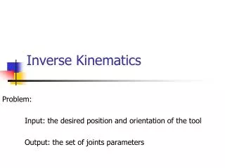
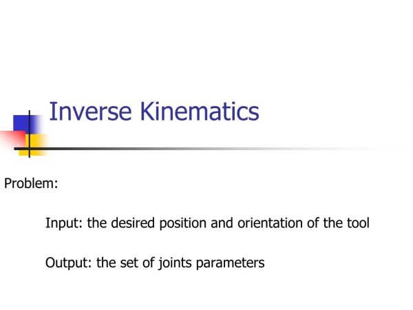
Inverse Kinematics • The goal of inverse kinematics is to compute the vector of joint DOFs that will cause the end effector to reach some desired goal state • In other words, it is the inverse of the forward kinematics problem
Inverse Kinematics Issues • IK is challenging because while f() may be relatively easy to evaluate, f-1() usually isn’t • For one thing, there may be several possible solutions for Φ, or there may be no solutions • Even if there is a solution, it may require complex and expensive computations to find it • As a result, there are many different approaches to solving IK problems
Analytical vs. Numerical Solutions • One major way to classify IK solutions is into analytical and numerical methods • Analytical methods attempt to mathematically solve an exact solution by directly inverting the forward kinematics equations. This is only possible on relatively simple chains. • Numerical methods use approximation and iteration to converge on a solution. They tend to be more expensive, but far more general purpose. • Today, we will examine a numerical IK technique based on Jacobian matrices
Derivative of a Scalar Function • If we have a scalar function f of a single variable x, we can write it as f(x) • The derivative of the function with respect to x is df/dx • The derivative is defined as:
Derivative of a Scalar Function f(x) Slope=df/dx f-axis x-axis x
Exact vs. Approximate • Many algorithms require the computation of derivatives • Sometimes, we can compute analytical derivatives. For example: • Other times, we have a function that’s too complex, and we can’t compute an exact derivative • As long as we can evaluate the function, we can always approximate a derivative
Approximate Derivative f(x+Δx) f(x) Slope=Δf/Δx f-axis x-axis Δx
Nearby Function Values • If we know the value of a function and its derivative at some x, we can estimate what the value of the function is at other points near x
Finding Solutions to f(x)=0 • There are many mathematical and computational approaches to finding values of x for which f(x)=0 • One such way is the gradient descent method • If we can evaluate f(x) and df/dx for any value of x, we can always follow the gradient (slope) in the direction towards 0
Gradient Descent • We want to find the value of x that causes f(x) to equal 0 • We will start at some value x0 and keep taking small steps: xi+1 = xi + Δx until we find a value xN that satisfies f(xN)=0 • For each step, we try to choose a value of Δx that will bring us closer to our goal • We can use the derivative as an approximation to the slope of the function and use this information to move ‘downhill’ towards zero
Gradient Descent df/dx f(xi) f-axis xi x-axis
Minimization • If f(xi) is not 0, the value of f(xi) can be thought of as an error. The goal of gradient descent is to minimize this error, and so we can refer to it as a minimization algorithm • Each step Δx we take results in the function changing its value. We will call this change Δf. • Ideally, we could have Δf = -f(xi). In other words, we want to take a step Δx that causes Δf to cancel out the error • More realistically, we will just hope that each step will bring us closer, and we can eventually stop when we get ‘close enough’ • This iterative process involving approximations is consistent with many numerical algorithms
Choosing Δx Step • If we have a function that varies heavily, we will be safest taking small steps • If we have a relatively smooth function, we could try stepping directly to where the linear approximation passes through 0
Choosing Δx Step • If we want to choose Δx to bring us to the value where the slope passes through 0, we can use:
Gradient Descent df/dx f(xi) f-axis xi+1 xi x-axis
Solving f(x)=g • If we don’t want to find where a function equals some value ‘g’ other than zero, we can simply think of it as minimizing f(x)-g and just step towards g:
Gradient Descent for f(x)=g df/dx f(xi) f-axis xi+1 g xi x-axis
Taking Safer Steps • Sometimes, we are dealing with non-smooth functions with varying derivatives • Therefore, our simple linear approximation is not very reliable for large values of Δx • There are many approaches to choosing a more appropriate (smaller) step size • One simple modification is to add a parameter β to scale our step (0≤ β ≤1)
Inverse of the Derivative • By the way, for scalar derivatives:
Stopping the Descent • At some point, we need to stop iterating • Ideally, we would stop when we get to our goal • Realistically, we will stop when we get to within some acceptable tolerance • However, occasionally, we may get ‘stuck’ in a situation where we can’t make any small step that takes us closer to our goal • We will discuss some more about this later
Derivative of a Vector Function • If we have a vector function r which represents a particle’s position as a function of time t:
Derivative of a Vector Function • By definition, the derivative of position is called velocity, and the derivative of velocity is acceleration
Vector Derivatives • We’ve seen how to take a derivative of a scalar vs. a scalar, and a vector vs. a scalar • What about the derivative of a scalar vs. a vector, or a vector vs. a vector?
Vector Derivatives • Derivatives of scalars with respect to vectors show up often in field equations, used in exciting subjects like fluid dynamics, solid mechanics, and other physically based animation techniques. If we are lucky, we’ll have time to look at these later in the quarter • Today, however, we will be looking at derivatives of vector quantities with respect to other vector quantities
Jacobians • A Jacobian is a vector derivative with respect to another vector • If we have a vector valued function of a vector of variables f(x), the Jacobian is a matrix of partial derivatives- one partial derivative for each combination of components of the vectors • The Jacobian matrix contains all of the information necessary to relate a change in any component of x to a change in any component of f • The Jacobian is usually written as J(f,x), but you can really just think of it as df/dx
Partial Derivatives • The use of the ∂ symbol instead of d for partial derivatives really just implies that it is a single component in a vector derivative • For many practical purposes, an individual partial derivative behaves like the derivative of a scalar with respect to another scalar
Jacobians • Let’s say we have a simple 2D robot arm with two 1-DOF rotational joints: • e=[ex ey] φ2 φ1
Jacobians • The Jacobian matrix J(e,Φ) shows how each component of e varies with respect to each joint angle
Jacobians • Consider what would happen if we increased φ1 by a small amount. What would happen to e ? • φ1
Jacobians • What if we increased φ2 by a small amount? • φ2
Jacobian for a 2D Robot Arm • φ2 φ1
Jacobian Matrices • Just as a scalar derivative df/dx of a function f(x) can vary over the domain of possible values for x, the Jacobian matrix J(e,Φ) varies over the domain of all possible poses for Φ • For any given joint pose vector Φ, we can explicitly compute the individual components of the Jacobian matrix
Jacobian as a Vector Derivative • Once again, sometimes it helps to think of: because J(e,Φ) contains all the information we need to know about how to relate changes in any component of Φ to changes in any component of e
Incremental Change in Pose • Lets say we have a vector ΔΦ that represents a small change in joint DOF values • We can approximate what the resulting change in e would be:
Incremental Change in Effector • What if we wanted to move the end effector by a small amount Δe. What small change ΔΦ will achieve this?
Incremental Change in e • Given some desired incremental change in end effector configuration Δe, we can compute an appropriate incremental change in joint DOFs ΔΦ Δe • φ2 φ1
Incremental Changes • Remember that forward kinematics is a nonlinear function (as it involves sin’s and cos’s of the input variables) • This implies that we can only use the Jacobian as an approximation that is valid near the current configuration • Therefore, we must repeat the process of computing a Jacobian and then taking a small step towards the goal until we get to where we want to be