Chapter 3 Image Enhancement in the Spatial Domain

1. Chapter 3Image Enhancement in the Spatial Domain • Image Enhancement in Spatial Domain

2. 3.1 Background • Spatial domain process on images can be described as g(x, y) = T[f(x, y)] • where f(x,y) is the input image, g(x,y) is the output image, T is an operator • T operates on the neighbors of (x, y) • a square or rectangular sub-image centered at (x,y) to yield the output g(x, y).

4. The simplest form of T is the neighborhood of size 11. • g depends on the value of f at (x, y) which is a gray level transformation as s = T(r) • where r and s are the gray-level of f(x, y) and g(x, y) at any point (x, y). • Enhancement of any point depends on that point only. • Point processing • Larger neighborhood provides more flexibility. • Mask processing or filtering

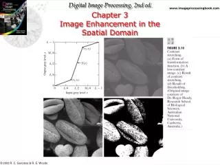
6. 3.2 Basic gray level transformations • Three basic functions used in image enhancement • Linear (negative and identity transformation) s = L-1-r • Logarithmic (log and inverse log) s = c log(1+r) • Power law (nth power and nth root transformation) s = cr or s = c(r+)

11.  correction • The CRT devices have an intensity-to-voltage response which is a power function. •  ranges from 1.8 to 2.5 • Without  correction, the monitor output will become darker than the original input.

14. Piecewise-Linear Transformation Functions • Contrast stretching

16. 3.3 Histogram Processing • The histogram of a digital image with gray-levels in the range [0, L-1] is a discrete function h(rk) = nk where rk is the kth level and nk is the number of pixels having the gray-level rk. • A normalized histogram h(rk)=nk/n, n is the total number of pixels in the image.

18. Histogram equalization is to find a transformation s = T(r) 0  r 1 that satisfies the following conditions: • T(r) is single-valued and monotonically increasing in the interval 0  r  1 • 0  T(r)  1 for 0  r  1 • T(r) is single-valued so that its inverse function exist.

20. The gray-level in an image may be viewed as a random variable, so we let pr(r) and ps(s)denote the probability density function of random variables r and s. • If pr(r)and T(r)are known and T-1(s) is single-valued and monotonically increased function then • Assume the transformation function as where w is a dummy variable, s = T(r)is a cumulative distribution function (CDF) of the random variable r.

21. Proof

22. For discrete case pr(rk) = nk/n for k = 0,1….L-1 • The discrete version of the transformation function is sk = T(rk)= • Advantage: • automatic, without the need for parameter specifications.

25. 3.3.2 Histogram Matching (Specification) • Given the input image with pr(r), and the specific output image withpz(z), find the transfer function between the r and z. • Let s = T(r) = • Define a random variable z with the property G(z) = = s • From the above equations G(z) = T(r) we have z = G-1(s) = G-1[T(r)]

26. For discrete case: • From given histogram pr(rk), k=0, 1,….L-1 sk = T(rk) = • From given histogram pz(zi), i=0, 1,…L-1 vk = G(zk) == sk • Finally, we have G(zk) = T(rk), and zk=G-1(sk)=G-1[T(rk)]

27. Obtain the histogram of each given image. • Pre-compute a mapped level sk for each level rk. • Obtain the transformation function G from given p(z) • Precompute zk for each value sk using iterative scheme as follows: • To find zk = G-1(sk) = G-1(vk), however, it may not exist such zk. • Since we are dealing with integer, the closest we can get to satisfying G(zk) – sk = 0 • For each pixel in the original image, if the value of that pixel is rk, map this value to its corresponding levels sk; then map level sk into the final level zk.

29. 3.5 Spatial Filtering • Spatial filtering: using a filter kernel ( which is a subimage, w(x, y)) to operate on the image f(x,y). • The response R of the pixel (x, y) after filtering is R = w(-1, -1)f(x-1, y-1) +w(-1, 0)f(x-1, y)+….+w(0, 0)f(x, y)+….+w(1, 0)f(x+1, y)+w(1, 1)f(x+1, y+1) The output image g(x,y) is:

32. 3.6 Smoothing Spatial Filters Weighted Averaging

35. 3.6.2 Smoothing Spatial Non-linear Filters • Median Filter • The response is based on ordering (ranking) the pixels contained in the image area encompassed by the filter, and then replacing the value of the center pixel with the value determined by the ranking result • For certain noise, such as salt-and-pepper noise, median filter is effective.

37. 3.7 Sharpening Spatial Filters • Image averaging – low-pass filtering – image blurring –spatial integration • Image sharpening – high-pass filtering –spatial differentiation. • It enhances the edges and the other discontinuities • First order difference is f/x = f(x+1, y) - f(x, y) f/y = f(x, y+1) - f(x, y) • Second order difference 2f/x2 = f(x+1, y) + f(x-1, y) - 2f(x, y)

39. 3.7.2 Second order derivative for enhancement • Isotropic filter, rotational invariant- Laplacian 2f = 2f/x2 + 2f/y2 2f = [f(x+1,y)+f(x-1,y)+f(x, y+1)+f(x, y-1)]- 4f(x,y)

41. Image enhancement g(x,y)=f(x,y)  2f(x,y) g(x,y)=f(x,y) + 2f(x,y) • Unsharp masking fs(x,y)=f(x,y) - f*(x,y), where f*(x,y)is the blurred image. • High boost filtering fhb(x,y)=Af(x,y)-f*(x,y)=(A-1)f(x,y)+f(x,y)-f*(x,y) =(A-1)f(x,y)+fs(x,y) • Using Laplacian fhb(x,y)=Af(x,y)2f (x,y) fhb(x,y)=Af(x,y)+2f (x,y)

42. Shapening的結果可能會有負值；要做rescaling把灰階的範圍調回0~255Shapening的結果可能會有負值；要做rescaling把灰階的範圍調回0~255 • 找出最小值t；如果t<0，把所有的像素加上|t|。 • 找出最大值M：如果 M>255，重新計算每一點灰階p；p’=(p/M)x255 • p’代表最後的灰階值。

46. 3.7.3 First derivative for enhancement • f(x,y)=[Gx, Gy]=[f/x, f/y ] • f(x,y)=mag (f )=[Gx2, Gy2]1/2 =[(f/x)2+(f/y)2 ]1/2 • Robert operator Gx=f/x=z9-z5 Gy=f/y =z8-z6 f(x,y)= [(z9-z5)2, (z8-z6)2 ]1/2 =|z9-z5|+|z8-z6| Sobel operator f(x,y)=|z7+2z8+z9)-(z1+2z2+z3)| +|(z3+2z6+z9)-(z1+2z4+z7)|

48. 3.8 Combining Spatial Enhancement Methods