Image Enhancement Techniques in the Spatial Domain: A Comprehensive Overview

1. EELE 5310: Digital Image ProcessingLecture 2Ch. 3Eng. Ruba A. SalamahRsalamah @ iugaza.Edu

2. Image Enhancement in the Spatial Domain

3. 3.1 Background • 3.2 Some Basic Gray Level Transformations Some Basic Gray Level Transformations • 3.2.1 Image Negatives • 3.2.2 Log Transformations • 3.2.3 Power-Law Transformations • 3.2.4 Piecewise-Linear Transformation Functions • Contrast stretching • Gray-level slicing • Bit-plane slicing Lecture Reading

4. Process an image so that the result will be more suitable than the original image for a specific application. The suitableness is up to each application. A method which is quite useful for enhancing an image may not necessarily be the best approach for enhancing another images Principle Objective of Enhancement

5. 2 domains • Spatial Domain : (image plane) • Techniques are based on direct manipulation of pixels in an image • Frequency Domain : • Techniques are based on modifying the Fourier transform of an image • There are some enhancement techniques based on various combinations of methods from these two categories.

6. Good images • For human visual • The visual evaluation of image quality is a highly subjective process. • It is hard to standardize the definition of a good image. • A certain amount of trial and error usually is required before a particular image enhancement approach is selected.

7. Spatial Domain • Procedures that operate directly on pixels. g(x,y) = T[f(x,y)] where • f(x,y) is the input image • g(x,y) is the processed image • T is an operator on f defined over some neighborhood of (x,y)

8. Mask/Filter • Neighborhood of a point (x,y) can be defined by using a square/rectangular (common used) or circular subimage area centered at (x,y) • The center of the subimage is moved from pixel to pixel starting at the top left corner. (x,y)

9. Point Processing • Neighborhood = 1x1 pixel • g depends on only the value of f at (x,y) • T = gray level (or intensity or mapping) transformation function: s = T(r) • Where • r = gray level of f(x,y) • s = gray level of g(x,y) • Because enhancement at any point in an image depends only on the gray level at that point, techniques in this category often are referred to as point processing.

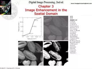
10. Contrast Stretching • Produce higher contrast than the original by: • darkening the levels below m in the original image • Brightening the levels above m in the original image

11. Thresholding • Produce a two-level (binary) image • T(r) is called a thresholding function.

12. Mask Processing or Filtering • Neighborhood is bigger than 1x1 pixel • Use a function of the values of f in a predefined neighborhood of (x,y) to determine the value of g at (x,y) • The value of the mask coefficients determine the nature of the process. • Used in techniques like: • Image Sharpening • Image Smoothing

13. Negative nth root Log nth power Output gray level, s Inverse Log Identity Input gray level, r 3 basic gray-level transformation functions • Linear function • Negative and identity transformations • Logarithm function • Log and inverse-log transformation • Power-law function • nth power and nth root transformations

14. Negative nth root Log nth power Output gray level, s Inverse Log Identity Input gray level, r Image Negatives • An image with gray level in the range [0, L-1]where L = 2n ; n = 1, 2… • Negative transformation : s = L – 1 –r • Reversing the intensity levels of an image. • Suitable for enhancing white or gray detail embedded in dark regions of an image, especially when the black area dominant in size.

15. Example: Image Negatives Original Negative

16. Negative nth root Log nth power Output gray level, s Inverse Log Identity Input gray level, r Log Transformations • c is a constant and r  0 • Log curve maps a narrow range of low gray-level values in the input image into a wider range of output levels. The opposite is true for higher values. • Used to expand the values of dark pixels in an image while compressing the higher-level values. s = c log (1+r)

17. Example of Logarithm Image

18. Negative nth root Log nth power Output gray level, s Inverse Log Identity Input gray level, r Inverse Logarithm Transformations • Do opposite to the Log Transformations • Used to expand the values of high pixels in an image while compressing the darker-level values.

19. Output gray level, s Input gray level, r Plots of s = cr for various values of  (c = 1 in all cases) Power-Law Transformations s = cr • c and  are positive constants • Power-law curves with fractional values of  map a narrow range of dark input values into a wider range of output values. The opposite is true for higher values of input levels. • c =  = 1  Identity function

20. Monitor  = 2.5 Gamma correction Monitor  =1/2.5 = 0.4 Example 1: Gamma correction • Cathode ray tube (CRT) devices have an intensity-to-voltage response that is a power function, with  varying from 1.8 to 2.5 • The picture will become darker. • Gamma correction is done by preprocessing the image before inputting it to the monitor with s = cr1/

21. Example 2: MRI (a) The picture is predominately dark (b) Result after power-law transformation with  = 0.6 (c) transformation with  = 0.4 (best result) (d) transformation with  = 0.3 (washed out look) under than 0.3 will be reduced to unacceptable level.

22. Example 3 (a) image has a washed-out appearance, it needs a compression of gray levels  needs  > 1 (b) result after power-law transformation with  = 3.0 (suitable) (c) transformation with  = 4.0 (suitable) (d) transformation with  = 5.0 (high contrast, the image has areas that are too dark, some detail is lost)

23. Piecewise-Linear Transformation Functions • Advantage: • The form of piecewise functions can be arbitrarily complex • Disadvantage: • Their specification requires considerably more user input

24. Contrast Stretching • increase the dynamic range of the gray levels in the image • (b) a low-contrast image • (c) result of contrast stretching: (r1,s1)=(rmin,0) and (r2,s2) = (rmax,L-1) • (d) result of thresholding

25. Gray-level slicing • Highlighting a specific range of gray levels in an image • Display a high value of all gray levels in the range of interest and a low value for all other gray levels • (a) transformation highlights range [A,B] of gray level and reduces all others to a constant level (result in binary image) • (b) transformation highlights range [A,B] but preserves all other levels

26. Bit-plane 7 (most significant) One 8-bit byte Bit-plane 0 (least significant) Bit-plane Slicing • Highlighting the contribution made to total image appearance by specific bits • Suppose each pixel is represented by 8 bits • Higher-order bits contain the majority of the visually significant data • Useful for analyzing the relative importance played by each bit of the image

27. An 8-bit fractal image Example

28. 8 bit planes

29. 3.3 Histogram processing 3.3.1 Histogram Equalization 3.3.2 Histogram Specification 3.4 Enhancement Using Arithmetic/Logic Operations 3.4.1 Image Subtraction 3.4.2 Image Averaging Next lecture Reading