Color spaces
Color spaces. CIE - RGB space. HSV - space. CIE - XYZ space. L*A*B* - space. YUV, YIQ CMY, CMYK. CIE-XYZ Gamut. Only the area between R,G,B can be reproduced by R,G,B primaries. Considerations in determining the R,B,G primitives. Producing a wide range of colors

Color spaces
E N D
Presentation Transcript
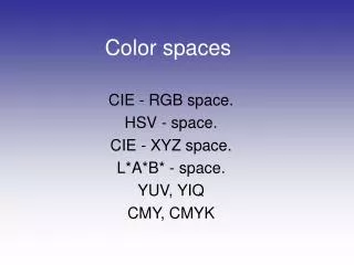
Color spaces CIE - RGB space. HSV - space. CIE - XYZ space. L*A*B* - space. YUV, YIQ CMY, CMYK
CIE-XYZ Gamut • Only the area between R,G,B can be reproduced by R,G,B primaries.
Considerations in determining the R,B,G primitives • Producing a wide range of colors • Dynamic range considerations: don’t use colors that you don’t need. • “System” considerations: Colors that are easy to produce by color monitors.
cian paint The CMY(K) model
Perceptual Models • L*ab color space normalizes the color space such that Euclidian distances will fit the perceptual ones (using JND) • For example: Human vision has a nonlinear perceptual response to brightness. • In general, I needed for just noticeable difference (JND) over background I was found to satisfy: I /I = const • Weber’s low: lightness perception is roughly logarithmic. • This is comparable to the L* component of the perceptual L*ab color model:
Color segmentation First try Segment the image according to its color histogram- Find “Clusters” of colors in the RGB space (or make a color quantization) Problem: In the RGB space, there is information which is not relevance to the chromaticity: lightening, texture and shadows. We need to eliminate the intensity !
Color segmentation (cont’) Solution: Convert the RGB image to another image space containing an intensity component- omit this component from the segmentation process. Examples: YIQ: Omit Y HSV (Hue, Saturation, Value): Omit V Original image Color segmentation using the HSV model
Skin Color Task: We would like to detect faces according to their color histograms Skin Color: The chromaticity of skin is very restricted (mainly the “Hue” component )* [*Skin Color is due to the amount of the pigment melanin]
Skin Color (cont’) Hue: Saturation: Value:
White balancing Problem: The color image is effected by the color of the light. Example: Outdoor scenes are “more blue” than indoor scenes. Possible solution: (far from perfect) Perform white balancing: find “white” regions, and change the color map such that these regions will become real white. Sometime, color skin can also be used for this purpose.
Geometry Surface albedo Viewing Lighting Image Simplified Physical Model: • An image is a function of many parameters:
Simplified Physical Model: • It is common to divide it into Lambertian components and specular ones. • Lambertian: The light is returned to all direction. • Specular: The light is returned in approx’ one direction. • Most objects are mainly Lambertian, but have a small Specular component.
Simplified Physical Model: • For Lambertian objects, the specular component is zero therefore we have a linear function. • Pixels belonging to a region with homogenous color should lie upon a line throw the origin in the RGB histogram. • With the Specular component, these pixels will lie on a plane (but most of the pixels will still lie on the original line)
The T-Shape model. • The T shape model introduced by Klinker et al. is widely used to model specularity. • The model assumes a large n in the previous equation => for each pixel there is only one dominant component
The color line model An ongoing work of Ido Omer and Mike Werman.
“Real Histogram” properties. • The lines best describing the color clusters don’t intersect the origin.
Cut Off: • One of the possible causes for the inaccuracy of the linear model is the “cut off “ phenomena in image sensors.
Comparing color segmentation using different color models. Original Lab HSV Color Lines
Color segmentation with “color lines” • slice the histogram perpendicularly to the origin. • search for local maxima. • combine these maxima to color lines
Color segmentation with “color lines” • Since we look only at the histogram, we are not effected by local image properties like texture. • The number of colors in the original image > 80,000, yet it has been described using ~40 lines. • Conclusion: The color histograms of natural images are very sparse.
Other distortions… Be aware: Most cameras apply various color enhancements that distorts the linear color model.
Talking about mosaicing, the “opposite” problem also exists. • Most digital cameras use filter arrays to sample red, green, and blue according to the Bayer pattern or similar ones. • At each pixel only one color sample is taken, and the values of the other colors must be interpolated from neighboring samples.
Demosaicing. • Many demosaicing techniques refer to the green channel as the “detail channel “ and to the red/blue channels as chrominance channels. • These techniques start by interpolating green values and then interpolate red/blue values according to the green one.