Input/Output Organization: Secondary Storage
This document dives into the complexities of binary prefixes in computing, highlighting the impact of standardization by the International Electrotechnical Commission (IEC) and the IEEE. It clarifies the confusion between binary and decimal measurements of storage, defining terms like kibibyte and mebibyte. Additionally, it explores the structure and functioning of magnetic hard disks, including components like disk geometry, seek time, and the Winchester technology that enhances data density. Understanding these concepts is essential for anyone dealing with secondary storage in computing.

Input/Output Organization: Secondary Storage
E N D
Presentation Transcript
Input/Output Organization:Secondary Storage CE 140 A1/A2 8 August 2003
Side Bar: Binary Prefixes • Before: Since 2^10 = 1024 ≈ 1000 = 1 kilo, 1024 bytes was referred to as 1 KB – OK at first • Problem: Confusion • 1 MB = 220 = 1,048,576 bytes • 1 MB = 106 = 1,000,000 bytes (storage industry) • 1 MB = 1,024,000 bytes (floppy disk) • For 1 GB, difference is about 7% • Solution: standardize the prefixes
Side Bar: Binary Prefixes December 1998: International Electrotechnical Commission (IEC), organization for worldwide standardization in electrotechnology approved a standard on binary prefixes IEEE now also uses a similar standard on a trial basis
Side Bar: Binary Prefixes • Examples • 1 kibibit = 1 Kibit (IEEE 1 Kb) = 210 bit = 1024 bits • 1 kilobit = 1 kbit (IEEE 1 KB) = 1010bit = 1000 bits • 1 mebibyte = 1 MiB = 220byte = 1,048,576 bytes • 1 megabyte = 1 MB = 1020byte = 1,000,000 bytes
Secondary Storage • Primary or main memory cannot accommodate all programs at once • Also, much of main memory is volatile • Need for cheap, large, non-volatile storage secondary storage • Examples • Magnetic hard disks, optical disks, floppy disks, tape systems
Magnetic Hard Disks • One more disks mounted on a common spindle • Disks are placed in a rotary drive • Disks rotate at uniform angular speed • Read/Write head – magnetic yoke/coil
Magnetic Hard Disk • Writing • current pulses applied to magnetic coil • Magnetization of film in underneath head switches direction parallel to applied field • Reading • Change in magnetic field in vicinity of head induces voltage/current in coil • Only changes can be monitored
Magnetic Hard Disks Source: PC Guide <http://www.pcguide.com/ref/hdd/op/index-c.html>
Magnetic Hard Disk Source: Structured Computer Organization by Tanenbaum
Magnetic Hard Disk • If magnetization states are presented by 1’s and 0’s, a string of 1’s or 0’s will only induce voltage at start and end of string • Clock is needed to synchronize information • Before: clock stored on a separate track • Now: clock encoded together with data • Simple example: Manchester encoding
1 1 1 1 0 0 0 Manchester encoding • Phase encoding • Change in magnetization for each bit • Space for each bit must accommodate two changes in magnetization
Winchester Technology • Disks and heads are placed in sealed, air-filtered enclosures • This allows read/write heads to operate closer to magnetic surface allowing for increased density • All modern drives use Winchester Technology
Three Parts of a Disk System • Disk – disk platters • Disk Drive – electromechanical mechanism, includes rotary drive and read/write heads • Disk Controller – controls disk operation, may or may not be part of the disk enclosure
Physical Disk Geometry TRACK SECTOR
Physical Disk Geometry • Previous figure shows each track has same number of sectors, the number of sectors in each track is the same as the maximum number of sectors that can be placed in the innermost track • Zoned Bit Recording (ZBR) – varies the number of sectors per track so that each track can be utilized more efficiently
Physical Disk Geometry • Track – concentric divisions of the surface • Sector – divisions in the track • Cylinder – set of corresponding tracks on all surfaces; data on same cylinder can be accessed without moving read/write head • Three coordinates to locate data: surface number, track number, sector number
Physical Disk Geometry • CHS Geometry • C – number of cylinders (tracks per surface) • H – number of heads (number of surfaces) • S – number of sectors per track • OK for older disks • NOT OK for newer disks • Zoned Bit Recording • Defect Mapping • Disk controller needs translation mechanism
Sector • Usually stores 512 bytes of data • Consists of preamble or sector header • Error-correcting code (ECC) information at the end • Sectors are separated by intersector gaps
Magnetic Hard Disks Source: Structured Computer Organization by Tanenbaum
Formatting a Disk • Unformatted Disk: absolutely no information • Formatting divides disk into tracks and sectors • Unformatted Size > Formatted Size • 15% of disk size is taken up by formatting information
Access Time • Seek Time: time for the arm to be moved to the right radial position • Rotational latency/delay: time for the desired sector to rotate under the head • Seek Time + Rotational Delay = Disk Access Time
Hard Disk Example • 3.5” disk (usually found in desktop PCs) • 20 data-recording surfaces • 15,000 tracks per surface • 400 sectors per track • 512 bytes per sector • Total formatted capacity: 61,440,000,000 bytes = 57.2 GiB = 61.4 GB
Logical Disk Geometry • What’s wrong with previous example: • 20 data-recording surfaces = 10 platter? Most disks usually just have around 3 platters! • Because of BIOS limitations, disk controllers intentionally mis-represent their characteristics as a logical disk geometry, to overcome size barriers imposed by BIOS • Also, physical disk geometry is no longer practical with ZBR and defect mapping
Logical Block Addressing (LBA) • Alternative to CHS addressing • Overcomes BIOS size limitations • Each sector is just numbered from 0,1,2,3,4,… up • Disk controller just translates these LBA addresses to actual physical addresses
Data Buffer/Cache • If bus to which disk is connected is much faster than the disk, data buffer is needed (this is a standard I/O practice) • Data buffer can also serve as a cache to disk contents
Disk Controller • Controls operation of disk • Interface to the bus • OS initiated Read transfer: MM address, disk address, word count • Disk controller: Seek, Read, Write, Error Checking
Floppy Disks • Used as removable storage • The read/write head touches the magnetic surface higher failure rate • Disk is not continously spinning, only when accessed
Commercially Available Hard Disks • ATA/IDE Disks • Most popular on general-purpose PCs • SCSI Disks • For high-performance servers/workstations • RAID • For increased redundancy and reliability
Integrated Drive Electronics (IDE) • One of the first type of drives where the controller is integrated with the drive itself • Term is used to refer to ATA drives which leads to confusion because SCSI drives also have disk controllers integrated with the disk package • Before: controllers were in separate modules and hard disk-specific
ATA – Advanced Technology Attachment • Primary storage interface used in PCs • ATA drives are also sometimes referred to as IDE drives ATA/IDE drives • ATA is the correct term for the interface • Different versions of the ATA standard different speeds
ATA Size Barrier • 28 bits are used to specify a sector • 228 = 268,435,456 sectors • 512 bytes/sector 137.4 GB or 128 GiB • Solution: new ATA standard ATA-6 allows 48 bits to specify a sector • 248 = 281,474,976,710,656 sectors • 128 PiB or 144 PB
SCSI Disks • SCSI – Small Computer System Interface • Usually used as a storage interface in high-end machines • Generally provides better performance than ATA disks • Higher Cost: 9500 pesos for 18.4 GB SCSI (10K RPM) versus 5000 pesos for 80 GB ATA (7200 RPM)
RAID Disk Arrays • RAID – Redundant Array of Independent (previously Inexpensive Disks) • Original idea by Patterson et al - Patterson was same guy who started RISC • “Villain”: SLED – single large expensive disk
RAID Disk Arrays • Rationale: Provide more redundancy with the use of “cheap” disks • Reliability is highly important when with storage devices • Realiability versus Availability • Realiablity – is something broken? • Availability – is the system still available to the user?
RAID Disk Arrays • Increasing redundancy will not improve reliability, it can only improve availability • Increased performance: throughput is increased by having multiple drives/read-write heads accessing data at the same time • Drawback: an array with N devices will have 1/N the reliability of a single device
RAID Disk Arrays • When a single disk fails, lost information can be recovered from redundant information • DANGER: When another disk failure happens between a time a disk fails and the time it is replaced/repaired (MTTR – mean time to repair – measured in hours) • MTTF (mean time to failure) is measured in years • An array of disks has higher availability than a single disk
RAID Levels • RAID 0 • Simply interleaves strips of data over multiple disks • No redundancy! – not really a true RAID • RAID 1 • Mirrored data • Just copy data in backup drive in the event of a failure • RAID 2 • Interleaves bytes of data over multiple disks • Can use Hamming code • Example: 1 byte is divided into 2 nibbles (4 bits), 3 bits of Hamming code are added total 7 bits distributed among 7 drives • Needs disk arms to be synchronized
RAID Levels • RAID 3 • Similar to RAID 2 • But only 1 parity bit is added to every nibble • RAID 4 • Works with strips again • Parity is written to 1 drive • RAID 5 • Parity information is distributed among the different disks • Reduces bottleneck on parity drive in RAID 4
RAID Disk Arrays Source: Structured Computer Organization by Tanenbaum
Optical Disks • Data is stored using the application of light (optical) • First Generation: LaserVision from Philips used for movies (laser discs) • Next: Philips and Sony came up with the CD (Compact Disc) used for audio • CDs: 120 mm across, 1.2 mm thick, with a 15-mm hole, supposed to last 100 years
Aluminum Acrylic Polycarbonate Plastic Land Pit Cross-Section of Optical Disk Label
Transition from Pit to Land Pit Land No Reflection Reflection Reflection Source Detector
CD Technology Source: Structured Computer Organization by Tanenbaum
CD Technology • For audio to play at uniform rate, pits and lands must stream by at a constant linear velocity • Slower angular velocity at the outside compared to the inside tracks
CD Data Layout • Data is stored in blocks called sectors • Different sector formats • Mode 1 format • 1 byte/symbol is encoded using 14 bits (6 bits used as Hamming code for error correction) • 1 frame = 42 consecutive symbols (588 bits) • Each frame holds 192 data bits (24 bytes), remaining 396 bits used for error correction • 1 sector = 98 frames • 16-byte header/preamble • 2048 bytes of stored data in 1 sector • 288 bytes for error-correction for the sector
CD Data Reliability • Three separate error-correcting schemes • Within a symbol/byte • Within a frame • Within a CD-ROM sector • It takes 98 frames of 588 bits (7203 bytes) to carry a single 2048-byte payload 28% Efficiency
CD-ROM Capacity and Speed • Single-Speed (1X) 75 sectors/sec 150 KiB/s • 650 MiB of data for ordinary disk
CD-ROM Source: Structured Computer Organization by Tanenbaum
AT Attachment Packet Interface • ATAPI allows CD-ROM and tape devices to share the ATA bus with ordinary disk drives