Sampling Distributions
Sampling Distributions. How likely are the possible values of a statistic?. Part 1: the Sampling Distribution of the Sample Mean. Briefly: What have we covered?. We use statistical analysis to make inferences about a population. 2. Sample statistics can be used to make such inferences.


Sampling Distributions
E N D
Presentation Transcript
Sampling Distributions How likely are the possible values of a statistic?
Part 1: the Sampling Distribution of the Sample Mean Briefly: What have we covered? • We use statistical analysis to make inferences about a population. 2. Sample statistics can be used to make such inferences. 3. We also learned that probability distributions can be used to construct models of a population
Question Who recalls what a sample statistic is? In practice, sample statistics are numerical summaries of sample data such as mean, variance, standard deviation, and binomial proportion which are used to estimate population parameters. What was the definition of a population parameter? It is a numerical summary of a population which is almost always unknown.
Where are we headed? Briefly: 1. We want to develop the notion that a sample statistic is a random variable with a probability distribution. 2. Define a sampling distribution for a sample statistic. • Link the sampling distribution of the sample statistic to the • normal probability distribution. I remember that:
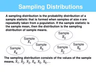
Question Before we proceed, does anyone know what a sampling distribution is or the definition? The concept of a sampling distribution is a little difficult for some students to understand. Basically, we have a population in which we could draw many different samples from the population. Sample 1 Sample 2 population Sample 3 Sample 4
Conjecture What is the result of being able to choose different samples in which to get a sample statistic? The sample statistic itself is a random variable. Thus, the sampling distributionof a sample statistic calculated from a sample of n measurements is the probability distribution of the statistic, that is, it is the probability distribution that specifies probabilities for the possible values the statistic can take. Moreover, sampling distributions describe the variability that occurs from study to study using statistics to estimate population parameters.
Sampling Distribution of the Sample Mean, is the probability distribution of all possible values of the random variable computed from a sample of size n from a population with mean and standard deviation . IMPORTANT: Even though we depend on sampling distribution models, we never actually get to see them. We never actually take repeated samples from the same population and make a histogram. We only imagine or simulate them.
Are you confused YET? Can we look at a simulation Wilber? You will find screen shots for the simulation on the next few slides.
Screen shots 1 Sample of size 5 drawn from population. Sample of size 5 drawn from population. Here are the five drawn from the population Here is their mean. Here are the means of the ten trials done. One trial of drawing a sample of size 5. Ten trials of drawing a sample of size 5.
Screen shots 2 Sample of size 30 drawn from population. Sample of size 30 drawn from population. One trial of drawing a sample of size 30. Notice how the means are more clustered for the trials that contained 30 subjects in each trial verses the ten trials in which the sample size was 5. Ten trials of drawing a sample of size 30.
Screen shots 3 Sample of size 30 drawn from population. Sample of size 5 drawn from population. 10000 trials of drawing a sample of size 5. 10000 trials of drawing a sample of size 30. Notice that the sampling distribution is more squashed in for the sample sizes of 30 verses 5
Thoughts What can you conclude when we take larger sample sizes? As we take larger sample sizes, the larger values are offset by smaller values giving us less spread in the sample means. In fact, the larger the sample size n, the more approximately normal the shape of the sample mean becomes. Why is it important for us to have a normal distribution? To be able to use previous results we have studied such as z-scores and the standard normal distribution.
Deviation in the Sampling Distribution Does anyone know what the standard deviation is called for a sampling distribution? The sampling distribution ofhas a standard deviation called the standard error in this case, the standard error of the sample mean, which gives us a mechanism to understand how much variability to expect in sample statistics that occur by chance. The standard error of the sample mean is given by: Where is the population standard deviation and n is the sample size. This holds for any size sample. Now do you understand why the size of n matters? As the size of n increases, so does the denominator which makes the standard error decrease! Moreover, the sample mean is more likely to fall closer to the population mean with a larger n.
Mean and Shape of the Sampling Distribution What about the sampling distribution mean? The sampling distribution of the sample mean will have mean: = µ Where µ is the population mean What about a population that is not normally distributed, how will that affect the sampling distribution of the mean ? This is when the Central Limit Theorem comes in.
Central Limit Theorem The Central Limit Theorem says that for a random sampling with a large size n, the sampling distribution of the sample mean is approximately normal. This result holds no matter what the shape of the distribution the samples were taken from. HOWEVER: The sampling distribution of the sample mean becomes more bell-shaped as the random sample size n increases. [Recall the example from earlier when n was 5 then 30.] The more skewed the population distribution, the larger the n must be for the shape of the sampling distribution is close to normal. Usually, the shape of the sampling distribution is usually close to normal when the sample size is at least 30.
Pause and Think Why is it important for us to be able to have a normal distribution for the sampling distribution when the population is not normally distributed? This enables us to make inferences about population means regardless of the shape of the population distribution. Let’s revisit the applet: Does the distribution to the right match any from the previous table?
Example 1 Suppose existing houses for sale average 2200 square feet in size, with a standard deviation of 250 square feet. What is the probability that a randomly selected house will have at least 2300 square feet? Strategy: Connect: Do you recall anything we have done that can help you set up this problem? We have used the standard normal distribution to find the probability that a given value is a specific amount. So we must standardize the value of 2300 square feet. Example 1
Calculate Here we have the value of x being greater than or equal to 2300 square feet. So we need to standardize this in order to use the standard normal distribution. We know the population mean and standard deviation, so we can find the z-value for x = 2300 square feet as we have done previously: Which here is: HOWEVER, this question is asking us to find the probability that x ≥ 2300 or: Example 1
Question What is the relevance of finding the z-value for the given value of 2300 ? Recall that the z-values tell us how many standard deviations away a value is from the mean. Here we are questioning the probability that 2300 is the lower bound for the size of a house randomly selected from a population whose mean size is 2200 with a standard deviation of 250 . Thus we need to find:
Visualize Recall that this area is .5. So to find the area you desire we must subtract the area for the z-value from table 4 from .5. What are we trying to calculate? This is the area I want to find. This is the probability that z ≥. 40 By table 4 this area for z = .40 is .1554
Calculate and Summarize Calculate Thus, by using table 4, we have that the Summarize: If a house is chosen at random from a group in which the average square footage is 2200 square feet with a standard deviation of 250 square feet, the probability that the house is greater than 2300 square feet is .3446 or 34.46%.
Key Think of the as an x valuelike we have dealt with previously. Then, as the sample size increases, by the Central Limit Theorem the sampling distribution that comes from becomes approximately normal. Thus we can use the z-value and normal distribution values (table 4) to find the probability that does….
Example 2 What is the probability that a randomly selected sample of 16 houses will average at least 2300 square feet? Strategy: Connect: How do we connect this problem to the previous problem? This is a similar problem BUT in this case we are asking the probability for a randomly selected sample of houses not just one house. Question:What do we know that can help to solve this problem? We know how to find the z-value of a given x, but here we are asked about the mean of one randomly selected sample of 16 houses that were chosen from the population of houses. Thus is a value that will fall within the sampling distribution of the sample mean. Thus by the Central Limit Theorem, I can find the z-value for .
Caution What is the one difference between calculating the z-value for and the z-value for a specific x? The difference is that instead of dividing by the population standard deviation, you have to divide by the standard error of which is the standard deviation divided by the square root of n. That is: = Think:What are we trying to find?
Calculate and Summarize : Thus for = 2300 with µ = 2200 and = = : Again by table 4 we must subtract the area of .4452 associated with the z-value of 1.60, to get: Summarize: The probability that a randomly selected sample of 16 houses will average a size greater than 2300 square feet given that the population of houses average 2200 square feet with a standard deviation of 250 square feet is .0548 or 5.48%.
You Try Water taxies have a safe capacity of 3500 lbs. Given that the population of men has normally distributed weights with a mean of 172 lb and a standard deviation of 29 lb, a) If one man is randomly selected, find the probability that his weight is greater than175 lb. Solution: Connect: How do the previous examples connect to this example? • Question: What do I know that will help me? • Think: Visualize what area or probability I am trying to find.
Calculate and Summarize The appropriate z-value, divide by the right quantity, i.e. Find the area for this z from table 4 which is .0398 Summarize: For a man chosen at random from the population of men with mean weight 172 lbs. and a standard deviation of 29lbs, the probability that the randomly chosen man weighs more than 172 lbs. is .4602 or 46.02%.
Second Part b) If 20 different men are randomly selected, find the probability that their mean weight is greater than 175 lb (so that their total weight exceeds the safe capacity for the water taxi of 3500 pounds). Strategy: Connect: How do the previous examples connect to this example? Question: What do I know that will help me? Think: Visualize what area or probability I am trying to find.
Calculate and Summarize The appropriate z-value, make sure you divide by the right quantity, i.e. Area for z = .46 from table 4 Summarize:Given that the safe capacity of the water taxi is 3500 pounds, there is a fairly good chance (with probability 0.3228) that it will be overloaded with 20 randomly selected men. Also notice that it is much easier for an individual to deviate from the mean than it is for a group of 20 to deviate from the mean.
You Try IQ scores are normally distributed with a mean of 100 and a standard deviation of 15. What is the probability a random sample of 20 people have a mean IQ score greater than 110? Mozart and Einstein were hypothesized to have IQs of about 4 standard deviations above the mean of 100.
Strategy • Connect: How do the previous examples connect to this example? • Question: What do I know that will help me? • Think: Visualize what area or probability I am trying to find. • Calculate: The appropriate z-value, divide by the right quantity, i.e. . • Summarize: • Answer: .0014
. Part 2: Sampling Distribution for the Sample Proportion What is the sampling distribution for the sample proportion? Like previously for the sampling distribution for the sample mean, it is a probability distribution of the sample proportion. The sample proportion is found by measuring if an individual either has or does not have a specific characteristic, this is a binomial variable. How is the sample proportion found? • We find a variable “p-hat” which is the proportion of the individuals in the sample with a specific characteristic we are interested in, x, divided by the number of individuals in the sample, n, . The sample proportion estimates the population proportion p.
Simulation AGAIN: This statistic will vary depending upon the sample taken from the population. Thus, this statistic is a binomial random variable as well. Each sample will vary with the number of individuals having the characteristic. Using the simulation we would have: This proportion is set so that 50% of the population has the interested characteristic so 50% does not. We selected 5 individuals randomly at a time In this random sample 2 individuals have the characteristic. I ran 1 trial. I ran another trial of 5 randomly selected individuals and only 1 had the characteristic. You can see the sampling distribution on the bottom now has 2 entries.
Screen shots 2 Notice what is happening as we take larger sample sizes and more trials.
Screen Shots 3 I set the probability of the population to 70 % has the characteristic in this case. IN ALL CASES no matter what the is as long as the sample size is large and enough trials are done, the sampling distribution of the sample proportion becomes approximatelynormal!!!
Summary: As the size of the sample, n, increases, the shape of the sampling distribution of the sample proportion becomes approximately normal. The standard deviation (standard error) of the sampling distribution of the sample proportion decreases as the sample size, n, increases. The mean of the sampling distribution of the sample proportion equals the population proportion, p.That is, the mean of the sample proportions is the population proportion. The expected value of the sample proportion is equal to the population proportion. Why is it important to be normal?! So we can use the z-values and normal distribution values (table 4).
Standard Error and Mean For the standard error Sampling distribution of the sample proportion will be approximately normal if np(1 - p) ≥ 10. For the mean
Example In a 2008 study : 85% of college students with cell phones use text messaging. 1136 college students surveyed; 84% reported that they text on their cell phone. Assume the value 0.85 given in the study is the proportion p of college students that text message; that is 0.85 is the population proportion p Compute the probability that in a sample of 1136 students, 84% or less, use text messaging.
Solution By table 4, z = -.94 has area .3264. Thus .5 - .3264 = .1736 Hence there is a 17.36% probability that 84% or less of college students use text message.
Summary of Sampling Distributions • This is the probability distribution of a sample statistic. • With random sampling, the sampling distribution provides probabilities for all the possible values of the statistic. • The sampling distribution provides the key for telling us how close a sample statistic falls to the corresponding unknown parameter. • Its standard deviation is called the standard error. • For random sampling with a large sample size n, by The Central Limit Theorem the sampling distribution of the sample mean is approximately a normal distribution. • This result applies no matter what the shape of the probability distribution from which the samples are taken. • In practice, the sampling distribution is usually close to normal when the sample size n is at least about 30, and for sample proportions np(1-p)≥10. • If the population distribution is approximately normal, then the sampling distribution is approximately normal for all sample sizes.