Sampling Distributions
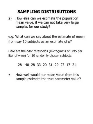
Sampling Distributions. Chapter 9. 9.1 Introduction. In real life calculating parameters of populations is prohibitive because populations are very large.

Sampling Distributions
E N D
Presentation Transcript
Sampling Distributions Chapter 9
9.1 Introduction • In real life calculating parameters of populations is prohibitive because populations are very large. • Rather than investigating the whole population, we take a sample, calculate a statistic related to theparameter of interest, and make an inference. • The sampling distribution of the statistic is the tool that tells us how close is the statistic to the parameter.
x 1 2 3 4 5 6 p(x) 1/6 1/6 1/6 1/6 1/6 1/6 9.2 Sampling Distribution of the Mean • An example • A die is thrown infinitely many times. Let X represent the number of spots showing on any throw. • The probability distribution of X is E(X) = 1(1/6) + 2(1/6) + 3(1/6)+ ………………….= 3.5 V(X) = (1-3.5)2(1/6) + (2-3.5)2(1/6) + …………. …= 2.92
Throwing a die twice – sample mean • Suppose we want to estimate m from the mean of a sample of size n = 2. • What is the distribution of ?
6/36 5/36 4/36 3/36 2/36 1/36 E( ) =1.0(1/36)+ 1.5(2/36)+….=3.5 V(X) = (1.0-3.5)2(1/36)+ (1.5-3.5)2(2/36)... = 1.46 1 1.5 2.0 2.5 3.0 3.5 4.0 4.5 5.0 5.5 6.0 The distribution of when n = 2
Notice that is smaller than sx. The larger the sample size the smaller . Therefore, tends to fall closer to m, as the sample size increases. Notice that is smaller than . The larger the sample size the smaller . Therefore, tends to fall closer to m, as the sample size increases. Sampling Distribution of the Mean
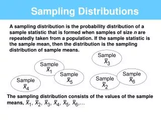
Sampling Distribution of the Mean Demonstration: The variance of the sample mean is smaller than the variance of the population. Mean = 1.5 Mean = 2. Mean = 2.5 1.5 2.5 Population 2 1 2 3 1.5 2.5 2 1.5 2 2.5 1.5 2 2.5 1.5 2.5 2 Compare the variability of the population to the variability of the sample mean. 1.5 2.5 1.5 2 2.5 1.5 2 2.5 1.5 2.5 2 1.5 2.5 1.5 2 2.5 1.5 2 2.5 Let us take samples of two observations 1.5 2 2.5
Sampling Distribution of the Mean Also, Expected value of the population = (1 + 2 + 3)/3 = 2 Expected value of the sample mean = (1.5 + 2 + 2.5)/3 = 2
The Central Limit Theorem • If a random sample is drawn from any population, the sampling distribution of the sample mean is approximately normal for a sufficiently large sample size. • The larger the sample size, the more closely the sampling distribution of will resemble a normal distribution.
Sampling Distribution of the Sample Mean • Example 9.1 • The amount of soda pop in each bottle is normally distributed with a mean of 32.2 ounces and a standard deviation of .3 ounces. • Find the probability that a bottle bought by a customer will contain more than 32 ounces. • Solution • The random variable X is the amount of soda in a bottle. 0.7486 m = 32.2 x = 32
0.7486 x = 32 m = 32.2 Sampling Distribution of the Sample Mean • Find the probability that a carton of four bottles will have a mean of more than 32 ounces of soda per bottle. • Solution • Define the random variable as the mean amount of soda per bottle. 0.9082
Sampling Distribution of the Sample Mean • Example 9.2 • Dean’s claim: The average weekly income of B.B.A graduates one year after graduation is $600. • Suppose the distribution of weekly income has a standard deviation of $100. What is the probability that 25 randomly selected graduates have an average weekly income of less than $550? • Solution
Sampling Distribution of the Sample Mean • Example 9.2– continued • If a random sample of 25 graduates actually had an average weekly income of $550, what would you conclude about the validity of the claim that the average weekly income is 600? • Solution • With m = 600 the probability of observing a sample mean as low as 550 is very small (0.0062). The claim that the mean weekly income is $600 is probably unjustified. • It will be more reasonable to assume that m is smaller than $600, because then a sample mean of $550 becomes more probable.
Using Sampling Distributions for Inference • To make inference about population parameters we use sampling distributions (as in Example 9.2). • The symmetry of the normal distribution along with the sample distribution of the mean lead to: - Z.025 Z.025
.95 .95 m=600 Using Sampling Distributions for Inference Standard normal distribution Z Normal distribution of .025 .025 .025 .025 Z m 0 -1.96 -1.96
Using Sampling Distributions for Inference • Conclusion • There is 95% chance that the sample mean falls within the interval [560.8, 639.2] if the population mean is 600. • Since the sample mean was 550, the population mean is probably not 600.
^ p The number of successes X n = 9.3 Sampling Distribution of a Proportion • The parameter of interest for nominal data is the proportion of times a particular outcome (success) occurs. • To estimate the population proportion ‘p’ we use the sample proportion. The estimate of p =
^ ^ p p 9.3 Sampling Distribution of a Proportion • Since X is binomial, probabilities about can be calculated from the binomial distribution. • Yet, for inference about we prefer to use normal approximation to the binomial.
Normal approximation to the Binomial • Normal approximation to the binomial works best when • the number of experiments (sample size) is large, and • the probability of success, p, is close to 0.5. • For the approximation to provide good results two conditions should be met: np 5; n(1 - p) 5
Normal approximation to the Binomial • Example • Approximate the binomial probability P(x=10) when n = 20 and p = .5 • The parameters of the normal distribution used to approximate the binomial are: • m = np; s2 = np(1 - p)
P(9.5<YNormal<10.5) The approximation ~ = P(9.5<Y<10.5) 9.5 10.5 Normal approximation to the Binomial Let us build a normal distribution to approximate the binomial P(X = 10). m = np = 20(.5) = 10; s2 = np(1 - p) = 20(.5)(1 - .5) = 5 s = 51/2 = 2.24 P(XBinomial = 10) = .176 10
4.5 13.5 Normal approximation to the Binomial • More examples of normal approximation to the binomial P(X £ 4) @ P(Y< 4.5) 4 P(X ³14) @ P(Y > 13.5) 14
Approximate Sampling Distribution of a Sample Proportion • From the laws of expected value and variance, it can be shown that E( ) = p and V( ) =p(1-p)/n • If both np > 5 and np(1-p) > 5, then • Z is approximately standard normally distributed.
Example 9.3 • A state representative received 52% of the votes in the last election. • One year later the representative wanted to study his popularity. • If his popularity has not changed, what is the probability that more than half of a sample of 300 voters would vote for him?
Example 9.3 • Solution • The number of respondents who prefer the representative is binomial with n = 300 and p = .52. Thus, np = 300(.52) = 156 andn(1-p) = 300(1-.52) = 144 (both greater than 5)
9.4 Sampling Distribution of the Difference Between Two Means • Independent samples are drawn from each of two normal populations • We’re interested in the sampling distribution of the difference between the two sample means
If the two populations are not both normally distributed, but the sample sizes are 30 or more, the distribution of is approximately normal. Sampling Distribution of the Difference Between Two Means • The distribution of is normal if • The two samples are independent, and • The parent populations are normally distributed.
We can define: Sampling Distribution of the Difference Between Two Means • Applying the laws of expected value and variance we have:
Sampling Distribution of the Difference Between Two Means Example 9.4 • The starting salaries of MBA students from two universities (WLU and UWO) are $62,000 (stand.dev. = $14,500), and $60,000 (stand. dev. = $18,3000). • What is the probability that a sample mean of WLU students will exceed the sample mean of UWO students? (nWLU = 50; nUWO = 60)
Sampling Distribution of the Difference Between Two Means • Example 9.4 – Solution We need to determine m1 - m2 = 62,000 - 60,000 = $2,000