Download
1 / 19
190 likes | 213 Vues
Research highlights methods for enhancing macromolecular dynamics understanding. It addresses issues such as kinetic model differentiation and parameter complexity. Techniques applied to study complex macromolecular systems.

E N D
Data Analysis Issues in Time-Resolved Fluorescence Anisotropy Bill Laws Department of Chemistry University of Montana Nick Vyleta, Abe Coley, Dawn Paul, Sandy Ross Support from NSF EPSCoR, NIH, and University of Montana
Correlations between parameters S b e -t/f • Saie -t/t j i j The Project • Enhance understanding of macromolecular • structure and function • Emphasis on rapid dynamics of small regions • that is, the kinetics of local motions • Requires a very fast measuring technique • such as time-resolved fluorescence anisotropy • Expand/develop methods in both data • collection and data analysis • Apply techniques to macromolecular systems The Issues • Differentiate numerous kinetic models that are very similar • Large number of iterated parameters • Multiple sets of acceptable values - - which is correct? • More complex systems even more parameters and kinetic models
Jablonski Diagram TimeScales Abs.: ~ 10 –15 s Si IC.: 10 –12 s Fluor: ~ 10 –9 s S3 Frank-Condon state S2 Internal Conversion S1 Fluorescence DE = hv = h/l Absorption S0 Fluorescence • A molecule has electronic, vibrational, • rotational, andtranslational energies • At room temperature, only rotational and • vibrational higher energy states will be • populated • Ground state: all electrons of molecule in • their lowest energy orbitals • Absorption: an electron acquires energy • (E1) from a photon, moving • it to a higher orbital • Excited state: the molecule with an electron • in a higher orbital • energy lost from molecular • reorganization (IC) • photochemistry may occur • Emission: molecule returns to ground state • as electron loses energy • by emitting a photon
Representative Spectra Absorbance Fluorescence Relative Intensity or Absorbance Wavelength (nm)
Time per collection of a data point is long (ms or greater) • Provides value proportional to the number of photons emitted in that time period • Fluorescence spectrum obtained by steady-state fluorescence • No kinetic information about the mechanism of fluorescence • Photon counting • Kinetics on the nanosecond time scale • Phase and modulation • Therefore need picosecond resolution for data Steady-State Fluorescence Time-Resolved Fluorescence
A* kf knr hv hv Typical lifetime of 1 to 100 ns Typical rates knr : 107 – 1010 s-1 kf : 107 – 109 s-1 Time-Resolved Fluorescence A
Representation of the Collection of a Decay Curve (t = 5 ns)
‘Time broadening’ due to response time of the instrumentation Counts Instrument Response Function (IRF) Time (ns)
t F(t) = ∫IRF(t - s) I(s) ds 0 Counts Time (ns) ‘Time broadening’ due to response time of the instrumentation Counts Instrument Response Function (IRF) Time (ns)
Collect both F(t) and IRF(t), and kinetic model yields decay function, I(t) • With ‘guestimates’, generate an initial fit by convolving I(t) with IRF(t) • Iterate parameters via non-linear least squares, minimizing reduced c2 n 1 sk2 c2 = S [Fc(k) – F(k)]2sk = [F(k)]1/2 1 n-p k=1 c2 c2 t F(t) = ∫ IRF(t - s) I(s) ds 0 parameter a t Data Fitting • Also use weighted residuals, autocorrelation of residuals, and parameter • confidence limits to evaluate fits
1 exp n m n 1 n 1 m Di = Fc(i) - F(i) wi = [1/F(t)] /S 1/F(t)] AC(j) = Swi1/2Di(wi+j)1/2Di+j/ Swi Di2 1 n i=1 i=1 i=1 S 2 exp S 3 exp Resid(t) = [Fc(t) - F(t)] / [F(t)]1/2 j from 1 to (n-m)
Photon absorption requires its E vector to align (cos2) with absorption dipole moment • Pulse of polarized light (vertical V) excites a defined population • If molecules ‘frozen’, only detect emitted photons with V polarization • If free to rotate, depolarization occurs and detect both V and H intensities • V and H intensities dependent on rates of depolarizing motions Steady-state anisotropy Time-resolved anisotropy IV – IH IV(t) – IH(t) r(t) = <r> = IV + 2 IH IV(t) + 2 IH(t) • <r> provides information on size, shape, and stability sample • r(t) provides the same information as well as • mechanism(s) of depolarization by kinetics laser polarizer rotate detector Fluorescence Anisotropy
Collect IM(t), IV(t), and IH(t) decays (along with each IRF) • These three decays constitute a dataset -t/t 1 3 IM(t) = a e t = f = 5 ns IM(t) -t/t IV(t) = a e {1 + 2 r(t)} IH(t) IV(t) – IH(t) IV(t) = -t/t IH(t) = a e {1 - r(t)} IV(t) + 2 IH(t) • One lifetime and one rotational correlation time • Iterating 12 parameters: a, t, b, f, 2 scalars, and 3 x 2 instrumental factors -t/f r(t) = b e • Simultaneous (global) analysis of the IM, IV, and IH dataset • Over determination of common parameters a, t, b, and f Our Anisotropy Method • Note: exponential times exponential
Sums of exponentials for intensity decay n -t/ti IM(t) = Sai e • Ground-state heterogeneity from multiple fluorophores and/or environments i = 1 • ai terms a function of several factors, including concentrations and spectral overlap m -t/fj r(t) = Sbij e • Sums of exponentials for anisotropy decay j = 1 Real World Complexities Lifetimes • Typical to require more than one lifetime (n > 1) • Resolution capabilities require t2 ~ 2t1; with a global analysis need ~20% difference • Although fits decay curve, correct kinetic model might not yield sums of exponentials Correlation Times • Likely to have more than one rotational correlation time (m > 1) • Different fj values for macromolecular rotations, segmental motions, and local motions • Resolution capabilities about a factor of 2; global analysis resolves ~40% difference • bi term is limiting anisotropy for fluorophore i at t = 0 - - must be between -0.2 and 0.4
n -t/ti IM(t) = Sai e i =1 1 3 m -t/fj ri(t) = S bij e n n -t/ti -t/ti j =1 IV(t) = Sai e {1 + 2 r(t)} IH(t) = Sai e {1 - r(t)} i =1 i =1 • Sums of exponentials times sums of exponentials m -t/fj S bij e } r(t) = • bij terms represent the association of a • fluorophore (i) with a depolarizing motion (j) • Large number of correlated parameters n j =1 -t/ti S{ai e n i =1 • Yields multiple sets of acceptable values -t/ti Sai e • If a bij term equals zero, fluorophore i • not depolarized by motion j i =1 Number of Kinetic Models (2n – 1)m • For our systems, all fluorophores • depolarized by macromolecular rotations • n • m 1 2 3 4 • 1 3 7 15 • 1 9 49 225 • 1 27 343 3375 • 1 81 2401 50625 • Difference in kinetic models will be from • segmental and local motions • Multiple kinetic models possible • Multiple models with different sets of • parameters can fit the data
m -t/fj ri(t) = Sbije j i12 Physical Associations Parameter Associations j = 1 Model t1f1 b11b12 Model Variables 0 b21b22 t2f2 t1f1 f1m1 f2m2 b11 0 1 0 b22 t2f2 t1f1 f1m1 f2m2 0 b12 2 b21 0 t2f2 t1f1 f1m1 f2m2 b11b12 3 0 0 t2f2 t1f1 f1m1 f2m2 0 0 4 b21b22 t2f2 t1f1 f1m1 f2m2 b11b12 5 b21 0 t2f2 t1f1 f1m1 f2m2 b11b12 1 1 1 1 1 1 1 1 1 6 0 b22 2 2 2 2 2 2 2 2 2 t2f2 t1f1 f1m1 f2m2 0 b12 7 b21b22 t2f2 t1f1 f1m1 f2m2 b11 0 8 b21b22 t2f2 Kinetic Models for a 2x2 Profile f1m1 f2m2
Kinetic Models for a 2 x 2 Profile j Model i 1 2 0 1 b11b12 2 b21b22 1 1 b11 0 2 0 b22 • Needed multiple (6) datasets collected • as a function of an independent variable 2 1 0 b12 2 b21 0 • Analysis of all datasets simultaneously (globally) 3 1 b11b12 2 0 0 • Best to vary ai, with ti, bij, and fj common 4 1 0 0 2 b21b22 • Iterating a minimum of 58 parameters • with a maximum of 8 common parameters 5 1 b11b12 2 b21 0 6 1 b11b12 2 0 b22 7 1 0 b12 2 b21b22 8 1 b11 0 2 b21b22 • Able to establish experimental and analysis methods • to differentiate models and recover parameters • First, used simulated data • Experimental verification of kinetic approach and • techniques for models 0, 1, 2, and 7
j M i 1 2 3 j M i 1 2 3 j M i 1 2 3 Kinetic Models for a 2 x 3 Profile 18 1 0 b12 0 2 b21b22b23 0 1 b11b12b13 2 b21b22b23 9 1 b11 0 b13 2 0 b22b23 19 1 0 b12b13 2 b21 0 b23 1 1 b11 0 0 2 0 b22b23 10 1 b11b12 0 2 0 b22b23 20 1 0 b12b13 2 b21b22 0 2 1 b11b12 0 2 0 0 b23 11 1 b11b12b13 2 0 0 b23 21 1 b11b12b13 2 b21b22 0 3 1 b11 0 b13 2 0 b22 0 12 1 b11b12b13 2 0 b22 0 22 1 b11b12b13 2 b21 0 b23 4 1 b11b12b13 2 0 0 0 13 1 b11 0 0 2 b21b22b23 23 1 b11b12b13 2 0 b22b23 5 1 0 b12b13 2 b21 0 0 14 1 b11 0 b13 2 b21b22 0 24 1 b11b12 0 2 b21b22b23 6 1 0 0 b13 2 b21b22 0 15 1 b11b12 0 2 b21 0 b23 25 1 b11 0 b13 2 b21b22b23 7 1 0 b12 0 2 b21 0 b23 16 1 b11b12b13 2 b21 0 0 26 1 0 b12b13 2 b21b22b23 8 1 0 0 0 2 b21b22b23 17 1 0 0 b13 2 b21b22b23
Current project needs at least a 2 x 3 profile • Cannot differentiate the 9 remaining models and non-physical parameters recovered • Multiple datasets as a function of an independent variable • Use of more than one independent variable • But some experimental systems do not have an independent variable • Reduce number of iterated parameters • Fix values if known from another experiment • Scale parameters wrt to an iterated one based on known ratio or model prediction • Data Analysis Issues HELP??? • Large number of iterated parameters • Correlations between parameters • Resolution of similar kinetic models • Minimum of 84 iterated parameters with a maximum of 12 common (assumes 6 datasets) • NSF proposal submitted to explore experimental approaches • Use <r> to restrict bij and fj values • Use <rx> = 0 to eliminate anisotropy of one fluorophore