Age structured populations
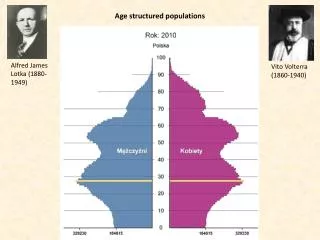
Age structured populations. Alfred James Lotka (1880-1949). Vito Volterra (1860-1940). First steps in life tables. Mortality rate. Survival rate. Fecundity. N 0 is the number of newborns. N is the number of females per age cohort.

Age structured populations
E N D
Presentation Transcript
Age structured populations Alfred James Lotka (1880-1949) Vito Volterra (1860-1940)
First steps in life tables Mortality rate Survival rate Fecundity • N0 is the number of newborns. • N is the number of females per age cohort. • Fecundity f is the average number of offspring per female. • d is the mortality rate per cohort. • l is the fraction of survivors per cohort.
Number of deaths at each age classage The pivotal age is the averge age per age cohort class Pivotal age The basic information needed is the total number of deaths per age cohort. survival mortality survival rate Mortality rate
First steps in life tables Death rate Survival rate Fecundity Population size of each cohort after reproduction Initial age distribution Age distribution of the next generation
If the population is age structured and contains k age classes we get Fecundities Survival rates Leslie matrix N0(0) = 1000 N0(1) = 1148 595*0.75=446 The mutiplication of the abundance vector with each row of the Leslie matrix gives the abundance of the next generation.
Leslie matrix We have w-1 age classes, w is the maximum age of an individual. L is a square matrix. Numbers per age class at time t+1 are the dot product of the Leslie matrix with the abundance vector N at time t The Leslie model is a linearapproach. It assumesstablefecundity and mortalityrates
Going Excel Demographic low • At the long run populationsizeincreases. • Diagonal waves in abundancesoccur. • The firstagecohortincreasesfastest.
The effect of age in reproduction Reproduction in early age contributes more to population size than later reproduction. This is caused by the higher number of females in earlier cohorts.
The effect of the initial age composition disappears over time • Age composition approaches an equilibrium although the whole population might go extinct. • Population growth or decline is often exponential High early death rates cause fast population extinction and would need high fecundities for population survival
Does the Leslie approach predict a stationary point where population abundances doesn’t change any more? We’re looking for the stable state vector that doesn’t change when multiplied with the Leslie matrix. This vector is the eigenvectorU of the matrix. Eigenvectors are only defined for square matrices. Important properties: Eventually all age classes grow or shrink at the same rate Initial growth depends on the age structure Early reproduction contributes more to population growth than late reproduction The largest eigenvalue l of a Leslie matrix denotes the long-term average net reproduction rate. The right (dominant) eigenvector contains the stable state age distribution.
Leslie matrices in insect populatons Largest eigenvalue r = l = 1.02 2000 female eggs per individual are cause a steady population increase. This relates to 4000 eggs when including males. Leslie matrices deal with effective populations sizes. Largest eigenvalue r = l = 0.65 The population steadily declines. The diagonal matrix elements show how many individuals survive.
Stable age distribution The largest eigenvalue l of a Leslie matrix denotes the long-term net population growth rate R. The right (dominant) eigenvector contains the stable state age distribution. For the population to survive the number of first instars has to be 0.189919/0.000398 = 477 time larger than the number of imagines. U = l = 1.02 Stable age class distribution
Remaining in the same age class The probability that an egg survives and remaines in the egg state is 0.10 The probability that an imago survives and reproduces in the next generation is 0.5. This is the case in biannual insects (for instance some Carabus) Largest eigenvalue R = l = 1.21 l = 1.21 l = 1.02 U= Without staying the same Stable age class distribution
Sensitivity analysis l = 1.14 l = 1.02 High mortality, high fecundity r strategist species Low mortality, low fecundity K strategist species l > 1 → effective population size increases How robust is l with respect to changes in survival and fecundity rates? l = 1.01 The lowest possible fecundity is 1.4 female eggs per female.
Sensitivity analysis l = 1.14 Increasing mortality rates until the population stops increasing l = 1.05 Mortality rates might be 10% higher to remain effective population sizes still increasing.
Survivorship tables Average number alive in a cohort Cumulative number alive in a cohort Death rate Number of death Average life expectation Survival rate k = length of cohort (10 years)
The female life table of Polishwomen 2012 (GUS 2013) Average life expectancyatbirth
Polish survivorship curve 2012 Type I Type I, high survivorship of young individuals: large mammals, birds Type II, survivorship independent of age, seed banks Type III, low survivorship of young individuals, fish, many insects Type II Type III Polish mortality rates 2012 Newborns New motocycle and car drivers
Average life expectancy at birth in Poland 81 years Women 8 years 72 years Men Average life expectancy at age 60 in Poland 84 years 5 years 78 years
Reproduction life tables Survival rate Number offspring R Birth rate Pivotal age The mean generation length is the mean period elapsing between the birth of parents and the birth of offspring. It is the weighted mean of pivotal age weighted by thenumber of offspring. Net reproduction rate
Life history data and body size Reproductive value at age x Life history data are allometrically related to body size. Data from Millar and Zammuto 1983, Ecology 64: 631
The characteristic life expectancy The Weibull distribution is particularly used in the analysis of life expectancies and mortality rates a=1 b=0.1b=0.5 b=1.0b=2.0b=3.0
We interpret the time t as the time to death. b > 1: Probability of death increases with timeb = 1: Probability of death is constant over timeb < 1: Probability of death decreases with time The two parameter Weibull probability density function Characteristic life expectancy T ; t = T 2.2 The characteristic life expectancy T is the age at which 63.2% of the population already died. F is the cumulative number of deaths.
How to estimate the characteristic life expectancy? Linearfunction Y = bX + C b = 0.95 C = -2.54 Type III survivorshipcurve
The female life table of Polish women 2012 (GUS 2013) Mortalities at younger age do not follow a Weibull distribution T = 86.8 years The characteristic life expectancy of Polish woman in 2012 was 87 years
The female life table of Polish women 2012 (GUS 2013) Maximum mortality 87 Mortality of newborns