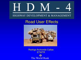
HDM-4 Road User Effects

1. HDM-4 Road User Effects

2. Road User Effects

3. RUE Research • Most models in use draw on HDM-III • No major RUE studies since HDM-III • Several studies addressed HDM-III calibration or investigated single components - e.g. fuel

4. Key Changes to HDM-III • Unlimited number of representative vehicles • Reduced maintenance and repair costs • Changes to utilization and service life modeling • Changes to capital, overhead and crew costs • New fuel consumption model • New oil consumption model • Changes to speed prediction model • Use of mechanistic tire model for all vehicles

5. New Features in HDM-4 • Effects of traffic congestion on speed, fuel, tires and maintenance costs • Non-motorized transport modeling • Traffic safety impact • Vehicle emissions impact

6. Motorcycle Small Car Medium Car Large Car Light Delivery Vehicle Light Goods Vehicle Four Wheel Drive Light Truck Medium Truck Heavy Truck Articulated Truck Mini-bus Light Bus Bicycles Rickshaw Animal Cart Pedestrian Representative Vehicles Motorized Traffic Non-Motorized Traffic • Medium Bus • Heavy Bus • Coach

7. Road User Costs Components • Fuel • Lubricant oil • Tire wear • Crew time • Maintenance labor • Maintenance parts • Depreciation • Interest • Overheads • Passenger time • Cargo holding time Vehicle Operating Costs Time Costs Accidents Costs

8. Vehicle Speed and Physical Quantities Roadway and Vehicle Characteristics Vehicle Speed Unit Costs Physical Quantities Road User Costs

9. Physical Quantities Component Quantities per Vehicle-km Fuel liters Lubricant oil liters Tire wear # of equivalent new tires Crew time hours Passenger time hours Cargo holding time hours Maintenance labor hours Maintenance parts % of new vehicle price Depreciation % of new vehicle price Interest % of new vehicle price

10. Free-Flow Speeds Model • VDRIVEu and VDRIVEd = uphill and downhill velocities limited by gradient and used driving power • VBRAKEu and VBRAKEd = uphill and downhill velocities limited by gradient and used braking power • VCURVE = velocity limited by curvature • VROUGH = velocity limited by roughness • VDESIR = desired velocity under ideal conditions Free speeds are calculated using a mechanistic/behavioral model and are a minimum of the following constraining velocities.

11. Free-Flow Speeds Model EXP( ^2/2)Vu = --------------------------------------------------------- 1 1/ 1 1/ 1 1/ 1 1/ 1 1/ (------) +(------) +(------) +(------) +(------) VDRIVEu VBRAKEu VCURVE VROUGH VDESIR EXP( ^2/2) Vd = --------------------------------------------------------- 1 1/ 1 1/ 1 1/ 1 1/ 1 1/ (------) +(------) +(------) +(------) +(------) VDRIVEd VBRAKEd VCURVE VROUGH VDESIR V = 2 / ( 1/Vu + 1/Vd ) Vu = Free-flow speed uphill Vd = Free-flow speed downhill V = Free-flow speed both directions = Sigma Weibull parameter = Beta Weibull parameter

12. Free-flow Speed and Roughness VBRAKE VCURVE VROUGH VDRIVE VDESIR Speed Curvature = 25 degrees/kmGradient = - 3.5 %

13. Free-flow Speed and Gradient VCURVE VBRAKE VROUGH VDRIVE VDESIR Speed Roughness = 3 IRI m/kmCurvature = 25 degrees/km

14. Free-flow Speed and Curvature VBRAKE VCURVE VROUGH VDRIVE VDESIR Speed Roughness = 3 IRI m/kmGradient = - 3.5 %

15. VDRIVE DriveForce Grade Resistance Air Resistance Rolling Resistance - Driving power- Operating weight- Gradient- Density of air- Aerodynamic drag coef.- Projected frontal area- Tire type- Number of wheels - Roughness- Texture depth- % time driven on snowcovered roads- % time driven on watercovered roads

16. For uphill travel, VBRAKE is infinite. For downhill travel, VBRAKE is dependent upon lengthof gradient. Once the gradient length exceeds a critical value,the brakes are used to retard the speed. - Braking power- Operating weight- Gradient- Density of air- Aerodynamic drag coef.- Projected frontal area- Tyre type- Number of wheels - Roughness- Texture depth- % time driven on snowcovered roads- % time driven on watercovered roads- Number of rise and fallper kilometers

17. VCURVE VCURVE is calculated as a function of the radius ofcurvature. VCURVE = a0 * R ^ a1 R = Radius of curvature R = 180,000/(*max(18/ ,C)) C = Horizontal curvature a0 and a1 = Regression parameters

18. VROUGH VROUGH is calculated as a function of roughness. VROUGH = ARVMAX/(a0 * RI) RI = Roughness ARVMAX = Maximum average rectified velocitya0 = Regression coefficient

19. VDESIR VDESIR is calculated as a function of road width, roadsidefriction, non-motorized traffic friction, posted speed limit, and speed enforcement factor. VDESIR = min (VDESIR0, PLIMIT*ENFAC)PLIMIT = Posted speed limit ENFAC = Speed enforcement factor VDESIR0 = Desired speed in the absence of posted speedlimitVDESIR0 = VDES * XFRI * XNMT * VDESMUL XFRI, XNMT = Roadside and NMT factors VDESMUL = Multiplication factor VDES = Base desired speed

20. Speeds Computational Logic • Calculate Free-Flow Speed for each vehicle type • Calculate the following for each traffic flow period: • Flow in PCSE/hr • Vehicle operating speed (Speed flow model) • Speed change cycle (Acceleration noise) • Vehicle operating costs • Travel time costs • Calculate averages for the year

21. Traffic Flow Periods To take into account different levels of traffic congestion at different hours of the day, and on different days of the week and year, HDM-4 considers the number of hours of the year (traffic flow period) for which different hourly flows are applicable. Flow Periods Flow Peak Nextto Peak Mediumflow NexttoLow Overnight Number of Hours in the Year

22. Passenger Car Space Equivalent (PCSE) To model the effects of congestion, mixed traffic flow is converted into equivalent standard vehicles. The conversion is based on the concept of ‘passenger car space equivalent’ (PCSE), which accounts only for the relative space taken up by the vehicle, and reflects that HDM-4 takes into account explicitly the speed differences of the various vehicles in the traffic stream.

23. Difference Between PCSE and PCU • PCU • consider two factors: • space occupied by vehicle • speed effects • used in highway capacity calculations • PCSE (HDM-4) • considers only space occupied • speed effects considered separately through speed model

24. PCSE Gap Length Space (m)

25. Speed Flow Model To consider reduction in speeds due to congestion, the “three-zone” model is adopted. Speed (km/hr) S1 S2 S3 S4 Sult Flow PCSE/hr Qnom Qo Qult

26. Speed Flow Model Qo = the flow below which traffic interactions are negligibleQnom = nominal capacityQult = ultimate capacity for stable flowSnom = speed at nominal capacity (0.85 * minimum free speed)Sult = speed at ultimate capacityS1, S2, S3…. = free flow speeds of different vehicle types Speed-Flow Model Parameters by Road Type

27. Speed Flow Types Speed (km/hr) Four Lane Wide Two Lane Two Lane Flow veh/hr

28. Roadside Friction

29. Fuel Model • Replaced HDM-III Brazil model with one based on ARRB ARFCOM model • Predicts fuel use as function of power usage

30. Implications of New Fuel Model • Lower rates of fuel consumption than HDM-III for many vehicles • Effect of speed on fuel significantly lower for passenger cars • Considers other factors – e.g. surface texture and type -- on fuel • Model can be used for congestion analyses

31. Effect of Speed on Fuel Consumption

32. Congestion - Fuel Model • 3-Zone model predicts as flows increase so do traffic interactions • As interactions increase so do accelerations and decelerations • Adopted concept of ‘acceleration noise’ -- the standard deviation of acceleration

33. Congestion Modelling

34. Effects of Speed Fluctuations(Acceleration Noise) • Vehicle interaction due to: • volume - capacity • roadside friction • non-motorised traffic • road roughness • driver behaviour & road geometry • Affects fuel consumption & operating costs

35. dFUEL Values by Acceleration Noise and Vehicle Speed

36. Effects Traffic Interactions on Fuel Consumption

37. Tire Consumption • Tread wear • amount of the tread worn due the mechanism of the tyre coming into contact with the pavement surface • Carcass wear • combination of fatigue and mechanical damage to the tyre carcass - affects number of retreads

38. Factors Influencing Tire Consumption

39. Effect of Congestion on Tyre Consumption

40. Parts and Labor Costs • Usually largest single component of VOC • In HDM-III user’s had choice of Kenya, Caribbean, India and Brazil models • All gave significantly different predictions • Most commonly used Brazil model had complex formulation • Few studies were found to have calibrated model

41. HDM-III (Brazil) Parts Consumption HDM-4Cars HDM-4Buses

42. Parts Model • Estimated from HDM-III Brazil model • Exponential models converted to linear models which gave similar predictions from 3 - 10 IRI • Roughness effects reduced 25% for trucks • For cars, roughness effects same as for trucks • For heavy buses, roughness effects reduced further 25%

43. Utilisation and Service Life • HDM-4 has either constant or ‘Optimal Life’ service life • Utilisation function of hours worked for work vehicles; lifetime kilometreage for private vehicles

44. Optimal Life Method • Proposed by Chesher and Harrison (1987) based upon work by Nash (1974) • Underlying philosophy is that the service life is influenced by operating conditions, particularly roughness • Relates life -- and capital costs -- to operating conditions

45. Optimal Life Method

46. Roughness and Lifetime Utilisation

47. Constant Service Life • Equations depend on the percentage of private use: • LIFEKM = LIFE x AKM < 50% • LIFEKM = S x HRWK x LIFE > 50%

48. Capital Costs • Comprised of depreciation and interest costs • HDM-III used a simple linear model affected by operating conditions through the effects of speed on utilization and service life • HDM-4 uses ‘Optimal Life’ method or constant life method

49. Depreciation in HDM-4 • Depreciation calculated multiplying the replacement vehicle price by the following equation: • The replacement vehicle price is reduced by a residual value which can be a function of roughness • The denominator is the lifetime utilisation which may be constant or predicted with the OL method to be a function of roughness

50. Roughness on Depreciation