Ordinary Differential Equations
CHAPTER 1. Ordinary Differential Equations. Contents. 1.1 Definitions and Terminology 1.2 Initial-Value Problems 1.3 Differential Equations as Mathematical Models. DEFINITION 1.1. Differential equation (DE). An equation contains the derivates of one or more dependent

Ordinary Differential Equations
E N D
Presentation Transcript
CHAPTER 1 Ordinary Differential Equations
Contents • 1.1 Definitions and Terminology • 1.2 Initial-Value Problems • 1.3 Differential Equations as Mathematical Models
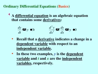
DEFINITION 1.1 Differential equation (DE) An equation contains the derivates of one or more dependent variables with respect to one or more independent variables. 1.1 Definitions and Terminology • Introduction: differential equations means that equations contain derivatives, eg:dy/dx = 0.2xy (1) • Ordinary DE: An eq. contains only ordinary derivates of one or more dependent variables of a single independent variable. eg: dy/dx + 5y = ex, (dx/dt) + (dy/dt) = 2x + y (2)
Partial DE: An equation contains partial derivates of one or more dependent variables of two or more independent variables. (3) • Notations: Leibniz notation dy/dx, d2y/ dx2 prime notation y’, y”, ….. Subscript notation ux, uy, uxx, uyy, uxy , …. • Order: highest order of derivatives first order second order
General form of n-th order ODE: (4) • Normal form of (4) (5)eg: normal form of 4xy’ + y = x, isy’ = (x – y)/4x • Linearity: An n-th order linear ODE can be expressed as
The following cases are for n = 1 and n = 2 and (7) • Two properties of a linear ODE:1) y, y’, y”, … are of the first degree.2) Coefficients a0, a1, …, depend at most on x • Nonlinear examples:
That is, a solution of (4) is a function possesses at least n derivatives and F(x, (x), ’(x),…, (n)(x)) = 0for all x in I, where I is the interval is defined on. DEFINITION 1.2 Solution of ODE Any function , defined on an interval I, possessing at least n derivatives that are continuous on I, when replaced into an n-th order ODE, reduces the equation into an identity, is said to be a solution of the equation on I.
Example 1 Verify the indicated function is a solution of the given ODE on (-, ) (a) dy/dx = xy1/2; y = x4/16(b) Solution :(a) Left-hand side: Right-hand side: then left = right (b) Left-hand side: Right-hand side: 0 then left = right
Suppose y = 0 is a solution of ODE, then y = 0 is called a trivial solution
Example 2 Function vs Solution y = 1/x, is the solution of xy’ + y = 0, however, this function is not differentiable at x = 0. So, the interval of definition I is (-, 0), or (0, ). Fig 1.1
DEFINITION 1.3 Implicit solution of an ODE G(x, y) = 0 is said to be an implicit solution of (4) on I, provided there exists at least one function y = (x) satisfying the relationship as well as the DE on I. • Explicit solution: dependent variable is expressed solely in terms of independent variable and constants.Eg: solution is y = (x).
Example 3 x2+ y2= 25 is an implicit solution of dy/dx = −x/y (8)on the interval -5 < x < 5. Since dx2/dx + dy2/dx = (d/dx)(25)then 2x + 2y(dy/dx) = 0 and dy/dx = -x/ysolution curve is shown in Fig1.2
Families of solutions: A solution containing an arbitrary constant c is called a one-parameter family of solutions. A solution containing n arbitrary constants c1, c2, …, cn is called a n-parameter family of solutions. • Particular solution: A solutionfree of arbitrary parameters. eg: y = cx – x cos x is a solution ofxy’ – y = x2sin x on(-, ), y = x cos x is a particular solution corresponding to c = 0. See Fig1.3
Example 4 x = c1cos 4t and x = c2 sin 4t are solutions ofx + 16x = 0we can easily verify that x = c1cos 4t + c2 sin 4t is also a solution.
Example 5 We can verify y = cx4 is a solution of xy – 4y = 0 on (-, ). See Fig1.4(a). The piecewise-defined function is a particular solution where we choose c = −1for x < 0and c = 1for x 0. See Fig1.4(b).
Singular solution: A solution can not be obtained by particularly setting any parameters. y = (x2/4 + c)2 is the family solution of dy/dx = xy1/2 , however, y = 0 is also a solution of the above DE. • We cannot set any value of c to obtain the solution y = 0, so we call y = 0 is a singular solution.
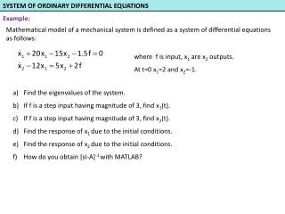
System of DEs: two or more equations involving two or more unknown functions of a single independent variable. dx/dt = f(t, x, y) dy/dt = g(t, x, y)(9)
1.2 Initial-value Problems • Introduction: We are often interested in a solution y(x) of a DE satisfying an initial condition. • Example: on some interval I containing xo, solve subject to (1)This is called an Initial-Value Problem (IVP). • y(xo) = yo , y(xo) = y1,are called initial conditions.
First and Second Order IVPs (2)and (3)are first and second order initial-value problems, respectively. See Fig1.7 and 1.8.
Example 1 We know y = cex is the solutions of y’ = y on (-, ). If y(0) = 3, then 3 = ce0 = c. Thus y = 3ex is a solution of this initial-value problem.If we want a solution passing through (1, -2), that is y(1) = -2, then -2 = ce, or c = -2e-1. See Fig1.9 Fig1.9
Example 2 In problem 6 of sec 2.2, we have the solution of y’ + 2xy2 = 0 to be y = 1/(x2 + c). If we impose y(0) = -1, it gives c = -1. Consider the following distinctions. 1) As a function, the domain of y = 1/(x2 - 1) is the set of all real numbers except -1 and 1. See Fig1.10(a). 2) As a solution, the intervals of definition are (-, -1) or (-1, 1) or (1, ) 3) As a initial-value problem, y(0) = -1, the interval of definition is (-1, 1). See Fig1.10
Example 3 In example 4 of Sec 1.1, we saw x = c1cos 4t + c2sin 4t is a solution ofx + 16x = 0Find a solution of the following IVP:x + 16x = 0, x(/2) = −2, x(/2) = 1 (4)Solution: Substitute x(/2) = − 2 into x = c1cos 4t + c2sin 4t, we find c1 = −2. In the same manner, from x(/2) = 1we have c2 = ¼.
Existence and Uniqueness:Does a solution of the IVP exist? If a solution exists, is it unique?
Example 4 Since y= x4/16and y = 0 satisfy the DEdy/dx = xy1/2 , and also initial-value y(0) = 0, this DE has at least two solutions, See Fig1.11 Fig1.11
THEOREM 1.1 Existence of a Unique Solution Let R be the region defined by a x b, c y d that contains the point (xo, yo) in its interior. If f(x, y) and f/y are continuous in R, then there exists some interval Io: xo- h < x < xo + h, h > 0, contained in a x b and a unique function y(x) defined on Io that is a solution of the IVP (2).
Fig1.12 • The geometry of Theorem 1.1 shows in Fig1.12
Example 5 For the DE: dy/dx = xy1/2 , we inspect the functionsand find they are continuous in y > 0. From Theorem 1.1, we conclude that through any point (xo, yo), yo> 0, there is some interval centered at xo on which this DE has a unique solution.
Interval of Existence and UniquenessSuppose y(x) is a solution of IVP (2), the following sets may not be the same: • the domain of y(x), the interval of definition of y(x)as a solution, the interval Io of existence and uniqueness.
1.3 DEs as Mathematical Models • Introduction:Mathematical models are mathematical descriptions of something. • Level of resolutionMake some reasonable assumptions about the system. • The steps of modeling process are as following
Assumptions Mathematics formulation Express assumptions in terms of differential equations If necessary, alter assumptions or increase resolution of the model Solve the DEs Obtain solution Check model Predictions with known facts Display model predictions, e.g., graphically
l + s unstretched x=0 x m equilibrium position mg – ks =0 l l in motion s m • Example: Spring/mass system • Observed from experiment: damping force ~ velocity • By Newton’s Law:
Series CircuitsLook at Fig1.21.From Kirchhoff’s second law, we have (11)where q(t) is the charge and dq(t)/dt = i(t), which is the current.