Download
1 / 16
160 likes | 494 Vues
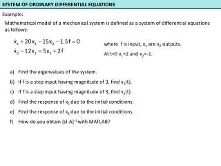
SYSTEM OF ORDINARY DIFFERENTIAL EQUATIONS. Example:. Mathematical model of a mechanical system is defined as a system of differential equations as follows:. where f is input, x 1 are x 2 outputs. At t=0 x 1 =2 and x 2 =-1. Find the eigenvalues of the system.

E N D
SYSTEM OF ORDINARY DIFFERENTIAL EQUATIONS Example: Mathematical model of a mechanical system is defined as a system of differential equations as follows: where f is input, x1 are x2 outputs. At t=0 x1=2 and x2=-1. • Find the eigenvalues of the system. • If f is a step input having magnitude of 3, find x1(t). • If f is a step input having magnitude of 3, find x2(t). • Find the response of x1 due to the initial conditions. • Find the response of x2 due to the initial conditions. • How do you obtain [sI-A]-1 with MATLAB?
SYSTEM OF ORDINARY DIFFERENTIAL EQUATIONS State Variables Form A B D(s) Let us obtain the State Variables Form so as to 1st order derivative terms are left-hand side and non-derivative terms are on the right-hand side.
SYSTEM OF ORDINARY DIFFERENTIAL EQUATIONS or Initial Conditions Solution due to the input Particular Solution Solution due to the initial conditions Homogeneous Solution General Solution clc;clear; num=[4.5 67.5]; den=[1 15 -280 0]; [r,p,k]=residue(num,den) a) Eigenvalues are roots of the polynomial D(s) or eigenvalues of the matrix A. b) x1(t) due to the forcing
SYSTEM OF ORDINARY DIFFERENTIAL EQUATIONS System is instable because of the positive root. Laplace transform of x2p clc;clear; num=[6 174]; den=[1 15 -280 0]; [r,p,k]=residue(num,den) c) x2(t) due to input
SYSTEM OF ORDINARY DIFFERENTIAL EQUATIONS clc;clear; num=[2 -25]; den=[1 15 -280]; [r,p,k]=residue(num,den) clc;clear; num=[-1 4]; den=[1 15 -280]; [r,p,k]= residue(num,den) f) [sI-A]-1 with Matlab. clc;clear; syms s; i1=eye(2) A=[-20 15;12 5]; a1=inv(s*i1-A) pretty(a1) d) x1 due to the initial conditions. e) x2 due to the initial conditions
SYSTEM OF ORDINARY DIFFERENTIAL EQUATIONS V2(t) 2 t (s) Example: • Mathematical model of a system is given below. Where V(t) is input, q1(t) and q2(t) are outputs. • Write the equations in the form of state variables. • Write Matlab code to obtain eigenvalues of the system. • Write Matlab code to obtain matrix [sI-A]-1. • Results of (b) and (c) which are obtained by computer are as follows: At t=0 and V(t) is a step input having magnitude of 2. Find the Laplace transform of due to the initial conditions. e) Find the Laplace transform of q1 due to the input.
SYSTEM OF ORDINARY DIFFERENTIAL EQUATIONS State variables B A a) State variables are q1, q2 and . System of differential equations is arranged so as to 1st order derivative terms are left-hand side and non-derivative terms are on the right-hand side. b) Matlab code which gives the eigenvalues of the system. A=[-1.5 1.5 0;0 0 1;3.75 -3.75 0]; eig(A) c) Matlab code which produces [sI-A]-1 clc;clear A=[-1.5 1.5 0;0 0 1;3.75 -3.75 0]; syms s; i1=eye(3); sia=inv(s*i1-A); pretty(sia)
SYSTEM OF ORDINARY DIFFERENTIAL EQUATIONS Example:Write the equation of motion of the mechanical system given below in the State Variables Form. Force applied on the system is F(t)=100 u(t) (a step input having magnitude 100 Newtons) and at t=0 x0=0.05 m and dx/dt=0. Find x(t) and v(t). State variables are x and v=dx/dt . m=20 kg c=40 Ns/m k=5000 N/m Matlab program to obtain eigenvalues: >>a=[0 1;-250 -2];eig(a)
SYSTEM OF ORDINARY DIFFERENTIAL EQUATIONS Applying Laplace transform and arranging, Solution due to the initial conditions Solution due to the input
SYSTEM OF ORDINARY DIFFERENTIAL EQUATIONS clc;clear; syms s; A=[0 1;-250 -2]; i1=eye(2); %unit matix with dimension 2x2 siA=s*i1-A; x0=[0.05;0]; %Initial conditions B=[0;0.05]; Fs=100/s; X=inv(siA)*x0+inv(siA)*B*Fs; pretty(X) For x(t) ; clc;clear; num=[0.05 0.1 5]; den=[1 2 250 0]; [r,p,k]=residue(num,den)
SYSTEM OF ORDINARY DIFFERENTIAL EQUATIONS Steady-state value (Final value) Initial value, x0
SYSTEM OF ORDINARY DIFFERENTIAL EQUATIONS For v(t) clc;clear; num=[-7.5]; den=[1 2 250]; [r,p,k]=residue(num,den)
SYSTEM OF ORDINARY DIFFERENTIAL EQUATIONS State variables Example: Mathematical model of a mechanical system having two degrees of freedom is given below. If F(t) is a step input having magnitude 50 Newtons, find the Laplace transforms of x and θ. R=0.2 m m=10 kg k=2000 N/m c=20 Ns/m
SYSTEM OF ORDINARY DIFFERENTIAL EQUATIONS clc;clear A=[0 0 1 0;0 0 0 1;-400 80 0 0;2000 -600 0 -2]; syms s; eig(A) i1=eye(4); sia=inv(s*i1-A); pretty(sia) System is stable since real parts of all eigenvalues are negative. Eigenvalues: If the initial conditions are zero, only the solution due to the input exists.