Functions of Random Variables

PROBABILITY AND STATISTICS FOR SCIENTISTS AND ENGINEERS Functions of Random Variables

Functions of Random Variables - Theorem X is a continuous random variable with probability distribution f(x). Let Y = u(X) define a one-to-one transformation between the values of X and Y so that the equation y = u(x) can be uniquely solved for x in terms of y, say x = w(y). Then the probability distribution of Y is: g(y) = f[w(y)]|J| where J = w'(y) and is called the Jacobian of the transformation

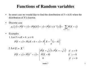
 a x axis x Example Consider the situation described by the figure. Assuming that the double arrow is spun so that  has a uniform density from -( /2) to  /2, suppose we want to find the probability density of x, the coordinate at the point to which the double arrow points. We are given The relationship between x and  is given by x = a tan , where a > 0.

Example Hence, and for -  < x <  and a>0 The probability density described below is called the Cauchy Distribution. It plays an important role in illustrating various aspects of statistical theory. For example, its moments do not exist. x 0

Linear Combinations of Random Variables If X1, X2, ..., Xn are independent random variables with means 1, 2, ..., nand standard deviations 1, 2, ..., n ,respectively , and if a1, a2, … an are real numbers then the random variable has mean and standard deviation (referred to as Root Mean Square, RSS)

Linear Combinations of Random Variables – Normal Distribution If X1, X2 ,…., Xn are independent normal random variables, where Xi ~ N(µi,σi) for i=1,2,…,n, and where ai is a real number, µi is the mean and σi is the standard deviation of Xi , for i=1,2,…,n then Y ~ N(µY,σY) where and

Linear Combinations of Random Variables Remark: This corollary is extremely important because it establishes a relationship between the important chi-squared and normal distributions. It also should provide a clear idea of what we mean by the parameter that we call degrees of freedom. Note that if Z1, Z2, ..., Zn are independent standard normal random variables, then X = has a chi-squared distribution and parameter, , the degrees of freedom, is n, the number of standard normal random variables.

Linear Combinations of Random Variables – Example Screws are packaged 100 per box. If individuals have weights that are independently and normally distributed with mean of 1 ounce and standard deviation of 0.5 ounce. What is the probability that a randomly selected box will weigh more than 110 ounces? What is the box weight for which there is a 1% chance of exceeding that weight? What would the per screw standard deviation have to be in order that the probability that a randomly selected box of screws will exceed 110 ounces is 5%?

Linear Combinations of Random Variables – Example Solution Since Xi ~ N(1,0.5) and

Linear Combinations of Random Variables – Example Solution then

Linear Combinations of Random Variables – Example Solution Therefore, Y ~ N(100, 5) a. P(Y > 110)

Linear Combinations of Random Variables – Example Solution Continued b. P(Y > c)

Linear Combinations of Random Variables – Example Solution Continued c. P(Y > 110) = 0.05 and

Linear Combinations of Random Variables – Example Solution Continued Since Therefore the standard deviation of the weight of a screw Is increased from to

Tolerance Limits - Example Consider the assembly shown. Suppose that the specifications on this assembly are 6.00 ± 0.06 in. Let each component x1, x2, and x3, be normally and independently distributed with means µ1 = 1.00 in., µ2 =3.00 in., and µ3 = 2.00 in., respectively. y x1m1=1.00 x2m2=3.00 x3m3=2.00

Tolerance Limits – Example Continued Suppose that we want the specifications to fall on the inside of the natural tolerance limits of the process for the final assembly such that the probability of falling outside of the specification limits is 7ppm. Establish the specification limits for each component.

Tolerance Limits - Example solution The length of the final assembly is normally distributed. Furthermore, if the allowable number of assemblies nonconforming to specifications is 7ppm, this implies that the natural limits must be located at m ± 4.49sy. (This value can be found on the normal distribution table in the resource section on the web site with a z-value of 0.0000035) That is, if  0.0134, then the number of nonconforming assemblies produced will be less than or equal to 7 ppm.

Tolerance Limits - Example Solution Continued Suppose that the variances of the component lengths are equal.

Tolerance Limits - Example Solution Continued This can be translated into specification limits on the individual components. If we assume natural tolerance limits, then So,

Packaging Problem - Example A company is having a packaging problem. The company purchases cardboard boxes nominally 10.5 inches in length intended to hold 4 units of a product they produced, stacked side by side in the boxes. Many of the boxes were unable to accommodate the 4 units so an objective was established to analyze the problem. Interns measured the thickness of 25 units of product. They found that these had a mean of 2.577 inches and a standard deviation of 0.061 inches. Also, they measured the inside of 25 boxes and found the inside lengths to have a mean of 10.367 inches and a standard deviation of 0.053 inches. Analysis indicated at the dimensions could be described by normal probability distributions.

Packaging Problem - Example The analysis objectives were to Determine the probability of the product (4 boxes) not fitting in a box Find a new target dimension for the inside length of the boxes ordered by the company so that only about 5% of the time 4 units will not fit inside the box.

Packaging Problem - Example Solution a) Let U = Y - (X1 + X2 + X3 + X4) where U is the clearance inside of the box Y is the inside box length Xi is the length of one unit for i = 1,2,3,4 Analysis of the measurement data indicates that the normal probability distribution provides a “good” fit to the data.Then

Packaging Problem - Example Solution Continued

Packaging Problem - Example Solution Continued So currently 33% will not fit into the box, which is bad.

Packaging Problem - Example Solution Continued b) Since Then

Linear Combinations of Random Variables – Special Cases The Poisson, the Normal and the Chi-squared distributions all possess the property that the sum of independent random variables having any of these distributions is a random variable that also has the same type of distribution.

Linear Combinations of Random Variables – Special Cases If X1, X2, ..., Xn are mutually independent random variables that have Chi-squared distributions with ν1, ν2, ..., νn degrees of freedom, then the random variable Y = X1 + X2 + ... + Xn has a Chi-squared distribution with ν = ν1+ ν2+ … + νn degrees of freedom.

Linear Combinations of Random Variables If X1, X2, ..., Xn are independent random variables having identical normal distributions with mean  and variance 2, then the random variable has a chi-squared distribution with = n degrees of freedom, since

Functions of Random Variables