Chapter 3 Discrete-Time Fourier Transform
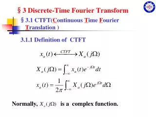
Chapter 3 Discrete-Time Fourier Transform. The Continuous-Time Fourier Transform. We already discussed this topic in Chapter 1. You can read this part( §3.1) in the textbook p117-122. Discrete-Time Fourier Transform.

Chapter 3 Discrete-Time Fourier Transform
E N D
Presentation Transcript
The Continuous-Time Fourier Transform • We already discussed this topic in Chapter 1. • You can read this part(§3.1) in the textbook p117-122.
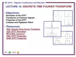
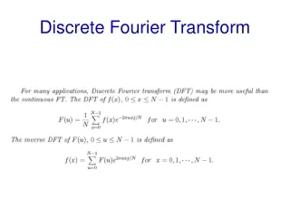
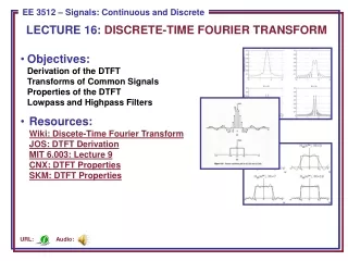
Discrete-Time Fourier Transform • Definition - The discrete-time Fourier transform (DTFT) X(ej) of a sequence x[n] is given by In general, X(ej) is a complex function of the real variable w and can be written as X(ej) = Xre(ej) + j Xim(ej)
Discrete-Time Fourier Transform • Xre(ej) and Xim(ej) are, respectively, the real and imaginary parts of X(ej) , and are real functions of w • X(ej) can alternately be expressed as X(ej) = | X(ej) |ej() where () = arg{X(ej) }
Discrete-Time Fourier Transform • | X(ej) | is called the magnitude function • () is called the phase function • Both quantities are again real functions of w • In many applications, the DTFT is called the Fourier spectrum • Likewise, | X(ej) | and () are called the magnitude and phase spectra
Discrete-Time Fourier Transform • For a real sequence x[n], | X(ej) | andXre(ej) are even functions of w, whereas, () and Xim(ej) are odd functions of w • Note: X(ej) = | X(ej) |ej(+2k) = | X(ej) |ej() for any integer k • The phase function q(w) cannot be uniquely specified for any DTFT
Discrete-Time Fourier Transform • Unless otherwise stated, we shall assume that the phase function q(w) is restricted to the following range of values: - q(w) called the principal value
Discrete-Time Fourier Transform • The DTFTs of some sequences exhibit discontinuities of 2p in their phase responses • An alternate type of phase function that is a continuous function of w is often used • It is derived from the original phase function by removing the discontinuities of 2p
Discrete-Time Fourier Transform • Example - The DTFT of the unit sample sequence d[n] is given by • Example - Consider the causal sequence
Discrete-Time Fourier Transform • Its DTFT is given by as
Discrete-Time Fourier Transform • The magnitude and phase of the DTFT X(ej) = 1/(1 – 0.5e-j) are shown below |X(ejω)|= |X(e-jω)| θ(ω)=-θ(-ω)
Discrete-Time Fourier Transform • The DTFT X(ej) of a sequence x[n] is a continuous function of w • It is also a periodic function of w with a period 2p:
Discrete-Time Fourier Transform • Therefore represents the Fourier series representation of the periodic function As a result, the Fourier coefficients x[n] can be computed from X(ej) using the Fourier integral
Discrete-Time Fourier Transform • Inverse discrete-time Fourier transform: Proof:
Discrete-Time Fourier Transform • The order of integration and summation can be interchanged if the summation inside the brackets converges uniformly, i.e. X(ej) exists • Then
Discrete-Time Fourier Transform • Now Hence
Some Basic properties of the Fourier Transform of a complex sequence • In general, the Fourier transform X(ejω) is a complex function of the real variable ωand can be written in rectangular form as X(ejω)= Xre(ejω) +j Xim(ejω) andXre(ejω) ={X(ejω)+ X*(ejω)}/2 Xim(ejω) ={X(ejω)- X*(ejω)}/2j also X(ejω)=| X(ejω)|ejθ(ω) θ(ω)=arg{X(ejω)}
Some Basic properties of the Fourier Transform of a complex sequence • The relations between the rectangular and polar forms of X(ejω) are given by: Xre(ejω) = | X(ejω)|cosθ(ω) Xim(ejω) = | X(ejω)|sinθ(ω) |X(ejω)|2=X(ejω)*X(ejω)=X2re(ejω)+X2im(ejω) tanθ(ω) = Xim(ejω) / Xre(ejω) Again X(ej) = | X(ej) |ej(+2k) = | X(ej) |ej()
Discrete-Time Fourier Transform • Convergence Condition - An infinite series of the form may or may not converge • Let
Discrete-Time Fourier Transform • Then for uniform convergence of X(ej) • Now, if x[n] is an absolutely summable sequence, i.e., if
Discrete-Time Fourier Transform • Then for all values of w • Thus, the absolute summability of x[n] is a sufficient condition for the existence of the DTFT X(ej)
Discrete-Time Fourier Transform • Example - The sequence x[n] = n[n] for ||< 1 is absolutely summable as and its DTFT X(ej) therefore converges to 1/(1- e-j) uniformly
Discrete-Time Fourier Transform • Since an absolutely summable sequence has always a finite energy • However, a finite-energy sequence is not necessarily absolutely summable
E Discrete-Time Fourier Transform • Example - The sequence has a finite energy equal to • But, x[n] is not absolutely summable
Discrete-Time Fourier Transform • To represent a finite energy sequence x[n] that is not absolutely summable by a DTFT X(ejω), it is necessary to consider a mean-square convergence of X(ejω): where
Discrete-Time Fourier Transform • Here, the total energy of the error X(ejω)- Xk(ejω) must approach zero at each value of ω as K goes to ∞ • In such a case, the absolute value of the error | X(ejω)- Xk(ejω)|may not go to zero as K goes to ∞ and the DTFT is no longer bounded
Discrete-Time Fourier Transform • Example: Consider the DTFT Shown below
Discrete-Time Fourier Transform • The inverse DTFT of HLP(ejω) is given by • The energy of hLP[n] is given by ωc/π • hLP[n] is a finite-energy sequence, but it is not absolutely summable
Discrete-Time Fourier Transform • As a result Does not uniformly converge to HLP(ejω) for all values of ω, but converges to HLP(ejω) in the mean-square sense
Discrete-Time Fourier Transform • The mean-square convergence property of the sequence hLP[n] can be further illustrated by examining the plot of the function For various values of K as shown in next slide
K=20 K=10 K=30 K=40 Discrete-Time Fourier Transform
Discrete-Time Fourier Transform • As can be seen from these plots, independent of the value of K there are ripples in the plot of HLP,K(ejω) around both sides of the point ω=ωc • The number of ripples increases as K increases with the height of the largest ripple remaining the same for all values of K
Discrete-Time Fourier Transform • As K goes to infinity, the condition holds indicating the convergence of HLP,K(ejω) approximation HLP (ejω) in the mean-square sense at a point of diccontinuity is known as the Gibbs phenomenon
Discrete-Time Fourier Transform • The DTFT can also be defined for a certain class of sequences which are neither absolutely summable nor square summable • Examples of such sequences are the unit step sequence μ[n], the sinusoidal sequence cos(ω0n+φ) and the exponential sequence Aαn • For this type of sequences, a DTFT representation is possible using the Dirac Delta function δ(ω)
w Discrete-Time Fourier Transform • A Dirac Delta function d(w) is a function of w with infinite height, zero width, and unit area • It is the limiting form of a unit area pulse function p() as D goes to zero satisfying
Discrete-Time Fourier Transform • Example - Consider the complex exponential sequence Its DTFT is given by where d(w) is an impulse function of w and
Discrete-Time Fourier Transform • The function is a periodic function of w with a period 2p and is called a periodic impulse train or impulse train • To verify that X(ej) given above is indeed the DTFT of x[n]=ej0n we compute the inverse DTFT of X(ej)
Discrete-Time Fourier Transform • Thus where we have used the sampling property of the impulse function()
Commonly Used DTFT Pairs Sequence DTFT
DTFT Theorems • There are a number of important properties of the DTFT that are useful in signal processing applications • These are listed here without proof • Their proofs are quite straightforward • We illustrate the applications of some of the DTFT properties
DTFT Theorems Type of Property Sequence DTFT g[n] G(ej) h[n] H(ej) Linearity ag[n]+bh[n] aG(ej)+bH(ej) Time-shifting g[n-n0] e-jn0G(ej) Frequency-shifting e-j0ng[n] G(ej(- 0)) Differentiation ng[n] jdG(ej)/d Convolution g[n]*h[n] G(ej)H(ej) Modulation g[n]h[n] Parseval’s relation
DTFT Theorems • g[n]←→G(ejω) • Use the definition of G(ejω)and differentiate both sides, we obtain The right-hand side of this equation is the Fourier transform of –jng[n]. Therefore, multiplying both sides by j, we see ng[n]←→jdG(ejω)/dω
DTFT Theorems • Example - Determine the DTFT Y(ej) of y[n]=(n+1)n[n], ||<1 Let x[n]=n[n], ||<1 • We can therefore write y[n]=nx[n] + x[n] • The DTFT of x[n] is given by
DTFT Theorems • Using the differentiation property of the DTFT, we observe that the DTFT of nx[n]is given by • Next using the linearity property of the DTFT we arrive at
DTFT Theorems • Example - Determine the DTFT V(ej) of the sequence v[n] defined by d0v[n]+d1v[n-1] = p0[n] + p1[n-1] • The DTFT of [n] is 1 • Using the time-shifting property of the DTFT we observe that the DTFT of [n-1] is e-j and the DTFT of v[n-1] is e-jV(ej)
DTFT Theorems • Using the linearity property we then obtain the frequency-domain representation of d0v[n]+d1v[n-1] = p0[n] + p1[n-1] as d0V(ej)+ d1e-jV(ej) = p0 + p1e-j • Solving the above equation we get
E E Energy Density Spectrum of a Discrete-Time Sequence • The total energy of a finite-energy sequence g[n] is given by • From Parseval’s relation we observe that
Energy Density Spectrum of a Discrete-Time Sequence • The quantity is called the energy density spectrum • The area under this curve in the range - divided by 2p is the energy of the sequence