Download
1 / 18
180 likes | 316 Vues
Gamma-ray Large Area Space Telescope. GLAST and pulsars: models and simulations. Massimiliano Razzano (INFN-Pisa). Astrofisica gamma dallo spazio in Italia AGILE e GLAST ESRIN, Frascati, 3 luglio 2007. PulsarSpectrum, simulating pulsars for GLAST. PulsarSpectrum simulator

E N D
Gamma-ray Large Area Space Telescope GLAST and pulsars:models and simulations Massimiliano Razzano (INFN-Pisa) Astrofisica gamma dallo spazio in Italia AGILE e GLAST ESRIN, Frascati, 3 luglio 2007 M.Razzano
PulsarSpectrum, simulating pulsars for GLAST PulsarSpectrum simulator Flexible architecture to allow creation of pulsar sources; Pulsar parameters easy to implement; PSRPhenom: Phenomenological model; PSRShape: Simulation of arbitrary energy-phase photon distribution; Simulation of timing effects; Full Interface with with LAT software (Gleam, observationSim);
PSRPhenom -Spectrum S(E) modeled with an analytical formula -Lightcurve L(f) independently created; • Nv (E,f) = k x L(f) x S(E); • Normalization k is specified by the user (Flux above 100 MeV); • Simple but some limitations PSRShape -Nv dependence on E and f is modeled using available data (EGRET) or prediction from theoretical models; More complex models and also phase-dependence of spectrum Creating the f-E histogram Photons from simulated pulsars are extracted according to a phase-energy distribution that is specified in a 2D ROOT histrogram (Nv) Nv histogram, that depend on the energy E and on the phase f, or equivalently time t Є[0,P]). 2 simulation schemes/models can be used for creating it.
Lightcurves can be random generated or read from a profile • Random curves (Lorentz peaks); • Existing TimeProfiles are useful for simulating known pulsars Random peaks Vela EGRET lightcurve (100 bins) Simulation model Lightcurve (2000 bins44us time bin width) PSRPhenom: simulating lightcurves
I choose this analytical spectral shape: (Nel and De Jager,1995): • Description of the high energy cutoff; • Parameters are obtained from fits on the known g ray pulsars (Nel, De Jager 1995); • Flux normalisation in a similar way to 3rdEGRET catalog (ph/cm2/s, E>100MeV); Different scenarios b=1 b=1.7 b=2 Example for Vela-like PSR F(E>100) ~9*10-6 ph/cm2/s, • En=1GeV,E0=8GeV; • g=1.62 Data from (N&DJ95) PSRPhenom: simulating spectra
PSRShape:simulating arbitrary models The base phenomenological model (power law + exp cutoff) cannot be used for more detailed phase-energy distribution of photons. A new model has been implemented • PSRShape features • External ROOT 2D histogram files can be used • Flux normalization can be adjusted; Resulting phase-dependent Vela (data from EGRET) Phase-dependent spectrum model based on EGRET data
Timing effects According to energy-phase distribution interval between photons are calculated, but the arrival times are processed for including timing effects. Timing analysis of pulsars is based on analysis steps for applying timing corrections (e.g. barycentering), and phase-assignment. Timing is affected by several effects. These effects must be considered in order to have a realistic list of photons arrival times. • Motion of GLAST in Solar System, relativistic effects (barycentering) • Period change with time; • Ephemerides and timing solutions; • Timing noise; • Modulation in case of binary pulsars;
Several effects that contribute to the barycentering, mainly: • Geometrical delays (due to light propagation); • Relativistic effects (i.e “Shapiro delay” due to gravitational wall of Sun) Time [days] Barycentric decorretions The analysis procedure on pulsars starts by perfoming the barycentering, i.e. transform the photon arrival times at the spacecraft to the Solar System Barycenter, located near the surface of the Sun In order to be more realistic for the simulations we then mustde-correct
Example of PN timing noise residuals for simulated pulsar called PSR J1734-3827 Adding Timing Noise Timing noise is an important issue since it affect lightcurves and pulsar blind searches. A basic model of timing noise is includes • Several studies and modeling have been proposed for timing noise; • For our purposes we choose the model based on Random Walk (Cordes 1980); Cordes Activity parameter A: • Noise events occurr at times ti • with mean rate R=1day-1 • k=0->Phase Noise, • k=1=Frequency Noise, • k=2,Slow down Noise
The Roemer delay can be seen, in this example of 6 months of sim. PSR J1735-5757 (Porb≈5.7 d) Pulsars in binary systems Emission from pulsars in binary systems could be much complicate. Since at this stage our purposes are mainly tests of SAE pulsar tools, we paid more attention to orbital motion than to pulsar emission processes • First stage implement Keplerian motions, including only: • Solution of Kepler’s equation; • Roemer delay; • Einstein and Shapiro delay already implemented, but no PPN parameters (e.g. g,r parameters) internally computed;
Filling the D4 file with simulated pulsars PulsarSpectrum is able to take both spin and orbital data of simulated pulsars for creating a D4 database gtpulsardb PulsarSpectrum • With simulations a summary file is created with names of files containing spin parameters and orbital parameters of the simulated pulsars; • These ASCII files can be converted into a single D4 fits file using gtpulsarb SimPulsars_summary.txt SimPulsars_spin.txt SimPulsars_bin.txt SimPulsars_names.txt D4 fits file
Lightcurve E>100 MeV Lightcurve E> 10 GeV, 15 photons Example of simulations Lightcurve E>100 MeV PSR B1706-44, 1 months simulation
Model Lightcurve Count map Spectrum Simulation of PSR B1951+32 30 days Sim. observation
DC2: Pulsar population Credits:Seth Digel • EGRET pulsars (6); • 3EG-coincident pulsars (39); • Isolated “Normal” pulsars RL or RQ, based on Slot Gap emission (140); • Millisecond pulsars RL or RQ based on Polar Cap (229);
Vela,30d Geminga,55d EGRET pulsars: lightcurves Vela,55d Seeing that pulsars does pulse…. Crab,55d
Low confidence High confidence LogN-LogS (see D.J.Thompson ’03) counts Flux 10-8 ph(>100 MeV) /cm2 s How many pulsars? Estimates from DC2 EGRET: 6 High Confidence, 3 Low Confidence
LAT studying high-energy cutoff Using XSpec the spectra have been recontructed for Vela pulsar using 2 different emission scenarios.
Conclusions • GLAST LAT will be a powerful instrument for studying g-ray pulsars; • Only 7 pulsars are known to emit in gamma-rays then statistics is poor; • Simulations are a powerful tools for several goals: help development of analysis tools and test new analysis techniques; • Study and design focused analyses (e.g. sensitivity); • Give rough estimates of LAT capabilities on pulsars; • Pulsar simulations reached a good level of detail; • DC2 and SCs contain large population of full-detail pulsars; • Ancillary tools have been developed for producing realistic population and sent to PulsarSpectrum; • Using PulsarSpectrum, new simulated pulsars will be added in the next simulation runs; • Help and support LAT SWG on pulsars with production of focused simulations