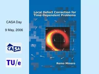
Adaptive Local Defect Correction for Transport of Passive Tracers in Time-Dependent Problems
180 likes | 299 Vues
This study presents the Local Defect Correction (LDC) method for solving time-dependent transport equations for passive tracers, such as pollutants. The LDC is an adaptive approach that combines coarse and fine grid solutions, enhancing accuracy in regions of high tracer activity. Key features include unconditionally convergent properties, multiple levels of refinement, and the ability to conserve tracer mass. The application to a dipole-wall collision problem illustrates the method’s effectiveness in modeling complex flow dynamics and tracer dispersion.

Adaptive Local Defect Correction for Transport of Passive Tracers in Time-Dependent Problems
E N D
Presentation Transcript
CASA Day 9 May, 2006
Outline • Transport of passive tracers • physical problem, mathematical model • Local Defect Correction (LDC) • basic method and its properties • extensions (conservation, multiple levels of refinement) • Numerical results Local Defect Correction for Time-Dependent Problems
Transport of passive tracer • Passive tracer: • a contaminant that does not influence the dynamics of the flow • Goal: • influence of the flow on the tracer • Applications: • dispersion of pollutants • mixing in chemical reactors Local Defect Correction for Time-Dependent Problems
Mathematical model • = distribution of passive tracerPe = Peclet numberv = given velocity field (or computed solving Navier-Stokes) • often has a local high activity • solve transport equation using Local Defect Correction (LDC) Local Defect Correction for Time-Dependent Problems
H h Local Defect Correction (LDC) • LDC: adaptive method for PDEs with highly localized properties • A coarse grid solution and a fine grid solution are iteratively combined Uniform structured grids Local Defect Correction for Time-Dependent Problems
t tn-1 tn t tn-1 tn t tn-1 tn One time step with LDC • Integrate on the coarse grid • Provide boundary conditions locally • Integrate on the local fine grid • Until convergence • Compute a defect at forward time • Solve a modified coarse grid problem • Provide new boundary conditions locally • Integrate on the fine grid with updated boundary conditions t tn-1 tn Δt δt Local Defect Correction for Time-Dependent Problems
Boundary conditions Coarse grid solution at tn Fine grid solution at tn Defect LDC iteration Local Defect Correction for Time-Dependent Problems
The defect • PDE • Coarse grid discretization • Fine grid solution is more accurate • Defect • Correction Local Defect Correction for Time-Dependent Problems
Properties of LDC • Convergence • Unconditionally convergent (i.e. for any Δt and H) • One or two iterations suffices • Convergence rate is O(Δt2 H-4)with implicit Euler + centered diff. • Limit solution satisfies where ΩlocH = common points between coarse and fine grid Local Defect Correction for Time-Dependent Problems
t tn tn-2 tn-1 Adaptivity • High activity can move • Locate high activity • Measure features of first coarse grid solution at tn • Provide initial values in the new fine grid points • Interpolate in space Local Defect Correction for Time-Dependent Problems
Conservation • Physical problem • if ·n = 0 and v·n = 0 on Ω, then tracer is conserved • A conservative LDC? • Combine LDC with Finite Volume • Defect • Scaling during regridding FINITE VOLUME ADAPTED LDC ALGORITHM: discrete conservation at convergence of the LDC iteration Local Defect Correction for Time-Dependent Problems
t tn-1 tn Multilevel LDC Local Defect Correction for Time-Dependent Problems
A dipole-wall collision problem • v from Navier-Stokes eq. in v- formulation in Ω = (0,2)x(-1,1) • boundary condition:v = 0 on Ω • initial condition: a dipole at the center • what happens: dipole travels, hits the wall, forms vortices (depending on Reynolds number) • solve by: spectral method • use: external Fortran code • Transport problem in Ω • boundary condition:·n = 0 on Ω • initial condition: tracer where the dipole hits the wall • what happens: tracer transported by v • solve by: FV adapted LDC with 2 levels of refinement & 1 LDC iteration/time step • use: C++ code Local Defect Correction for Time-Dependent Problems
Implementation of LDC class Problem { const Grid* g; const BoundaryConditions* bc; const InitialCondition* ic; const Defect* def; public: Problem(); void setGrid(const Grid* gg); void setBC(const BoundaryConditions* bbc); void setIC(const InitialCondition* iic); void setDef(const Defect* ddef); int solve(); /* some other stuff */ }; void provideBClocally( const Problem* global, Problem* local); void computeDefect( Problem* global, const Problem* local ); Local Defect Correction for Time-Dependent Problems
Numerical results: Re=250, Pe=500 Local Defect Correction for Time-Dependent Problems
Numerical results: Re=1250, Pe=2000 Local Defect Correction for Time-Dependent Problems
Conservation Total quantity of passive tracer LDC might be not fully converged in one iteration Local Defect Correction for Time-Dependent Problems
Conclusions • LDC is an adaptive method for solving PDEs • Coarse and fine grid solution iteratively combined • Extensions of the basic algorithm • conservative solution • multiple levels of refinement • LDC is applied to transport of passive tracers Local Defect Correction for Time-Dependent Problems