Understanding Probability and Uncertainty in Engineering Decision Making
Explore the math behind uncertainty in engineering decisions using probability theory. Learn about sets, distributions, Monte Carlo method, and stochastic analysis for deterministic and stochastic calculations.

Understanding Probability and Uncertainty in Engineering Decision Making
E N D
Presentation Transcript
Probability • Probability = mathematic interpretation of uncertainty • Uncertainty plays a major role in engineering decision making. • Set = collection of: • Items • Events • Occurrences • Distribution = behavior of a set
Monte Carlo Method • Statistic Analysis: • Have a set • Derive a distribution • Monte Carlo Method: • Have a distribution • Construct a model set
Example 1 Deterministic calculation of deflection for a cantilever beam with quadratic cross section: Deflection = 4 F L3 / E W H3 L = length of beam W = width of beam H = height of beam I = area moment of inertia E = Young’s modulus F = applied downward force
Example 1 Stochastic Calculation: Deflection = 4FL^3/EWH^3 • Symbols (physical parameters) represent distributions (expressed in MATLAB as vectors). • Vectors (distributions) should: • have the same number of elements • be randomly constructed according to preset rules regarding each quantity.
Common Distributions Uniform: Constant probability over a range of values. Useful for round-off errors Normal/Gaussian: Bell curve. Useful for large samples of random occurrences such as height.
Common Distributions Gamma: Only defined for positive x Useful for time dependant events, arrivals, etc. Exponential: A form of the Gamma, memory- less (events do not affect following occurrences) Weibull: A good representation of the frequency of failure for many types of equipment
Programs • Matlab • More than Matrices • Useful tool for Monte Carlo Modeling • Excel • Used to process results of Matlab models
Useful Commands in Matlab • R = unifrnd(A,B,m,n) generates uniform random numbers with parameters A and B, where scalars m and n are the row and column dimensions of R. • R = normrnd(MU,SIGMA,m,n) generates normal random numbers with parameters MU and SIGMA, where scalars m and n are the row and column dimensions of R. • R = gamrnd(A,B,m,n) generates gamma random numbers with parameters A and B, where scalars m and n are the row and column dimensions of R. • R = exprnd(MU,m,n) generates exponential random numbers with mean MU, where scalars m and n are the row and column dimensions of R. • R = wblrnd(A,B,m,n) generates Weibull random numbers with parameters A and B, where scalars m and n are the row and column dimensions of R.